2.1 Real Vector Spaces - ESE 2030 📏

1Reading¶

Material related to this page, as well as additional exercises, can be found in ALA Ch. 2.1 and LAA 4.1.

2Learning Objectives¶

By the end of this page, you should know:

the definition of a vector space
examples of different vector spaces
how to add and scale vectors

3Abstraction¶

A theme in mathematics is recognizing that seemingly unrelated settings, objects, or models, all share common properties. By viewing them at the right level of abstraction, they can all be reasoned about together in the same way. This is a very powerful way of thinking! This chapter will introduce the abstract notion of a vector space which unifies the seemignly disparate spaces of ordinary vectors, spaces of functions (such as polynomials, exponentials, and trigonometric functions), spaces of matrices, (infinite dimensional) linear operators (we will only briefly encounter these later in the course), and more under a common conceptual framework.

For many of you, this will be your first foray into “abstraction,” and it will take some time and effort to get used to these ideas. A good strategy is to make sure that you understand what the new concepts we introduce mean in the context of ordinary Euclidean space, and then work through how they might apply in more abstract spaces, like the space of polyomials, vector valued sampled signals over an interval, or symmetric matrices (yes, we will see that these are all examples of vector spaces!).

4Real Vector Spaces¶

We’ve so far relied on certain simple and intuitive algebraic properties of how matrices and vectors can be added together and scaled. We’ll try to formalize these ideas and then abstract/genearlize them next.

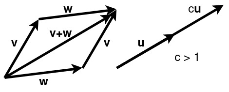
Let us consider the space of all $n \times 1$ real-values vectors, denoted by $\mathbb{R}^n$ . Adding two vectors $\vv v, \vv w \in \mathbb{R}^n$ can be viewed geometrically through a parallelogram, and multiplication by a scalar $c \in \mathbb{R}$ is stretching/shrinking the vector by factor $c$ .

We aim to abstract the above properties so that we can add and scale generic “vectors” living in a “vector space”.

Definition 1 (Vector Space Operations)

A vector space is a set $V$ equipped with two operations:

Addition: adding any pair of vectors $\vv v, \vv w \in V$ produces another vector $\vv v + \vv w \in V$ ,
Scalar Multiplication: multiplying a vector $\vv v \in V$ by a scalar $c \in \mathbb{R}$ produces a vector $c \vv v \in V$ .

These are subject to the following axioms, valid for all $\vv u, \vv v, \vv w \in V$ and all scalars $c, d \in \mathbb{R}$ :

Commutativity of Addition: $\vv v + \vv w = \vv w + \vv v$ .
Associativity of Addition: $\vv u + (\vv v + \vv w) = (\vv u + \vv v) + \vv w$ .
Additive Identity: There is a zero element $\vv 0 \in V$ satisfying $\vv v + \vv 0 = \vv v = \vv 0 + \vv v$ .
Additive Inverse: For each $\vv v \in V$ there is an element $− \vv v \in V$ such that $\vv v + (− \vv v) = \vv 0 = (− \vv v) + \vv v$ .
Distributivity: $( c + d) \vv v = (c \vv v) + (d \vv v)$ , and $c (\vv v + \vv w) = (c \vv v) + (c \vv w)$ .
Associativity of Scalar Multiplication: $c (d \vv v) = (c d) \vv v$ .
Unit for Scalar Multiplication: the scalar $1 \in \mathbb{R}$ satisﬁes $1 \vv v =\vv v$ .

The two operations just tell us that if we start with vectors $\vv v, \vv w \in V$ and real scalars $c, d \in \R$ , we are free to add scaled versions together and we will stay in the vector space $V$ , i.e., $c\vv v + d \vv w \in V$ for any choices of $c, d \in \R$ and $\vv v, \vv w \in V$ . The axioms that follow are a formalization of the properties we expect addition and multiplication to follow: these are true for ordinary numbers and ordinary vectors, and we want them to hold for generic vectors too. We will work through some familiar (and some not so familiar) examples soon, but we first highlight some additonal important properties that can be deduced from the axioms above.

Notice that these are all properties that obviously hold for ordinary numbers and ordinary vectors. The above says that these “rules” should also hold in our new abstract vector spaces.

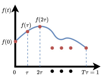
Example 3 (Sampled Functions over an Interval)

In digital signal processing and applications such as communication, we work with sampled versions of the functions $f(t)$ over the time interval $[0, 1]$ so that we can store them on a computer. This is obtained by sampling $f(t)$ at times $\{0, \tau, 2\tau, \ldots, T\tau = 1\}$ , where τ is the sampling period, and $\frac{1}{\tau} = T$ is the number of samples taken over $[0, 1]$ (we assume that τ is chosen so that $T$ is an integer).

This gives a vector of size $T+1$ :

\vv f = \bm f(0) \\ f(\tau) \\ f(2\tau) \\ \vdots \\ f(T\tau) \em.

(3)

So even though we started with a function defined over a continuous interval, after sampling it we end up with an ordinary vector of size $T+1$ . Hence, adding and scaling sampled functions is done in exactly the same way as in Example 1, but now the vectors $\vv f$ and $\vv g$ are interpreted as being samples from underlying functions $f(t)$ and $g(t)$ . Sampling the zero function $z(t) = 0$ gives the usual $\vv 0$ vector.

In summary, the space of functions sampled at the same $T+1$ time points over an interval is not only a vector space, but is in fact $\mathbb{R}^{T + 1}$ !

Example 4 (Doubly Infinite Sequences of Numbers

\mathbb{S}

)

Let $\mathbb{S}$ be the space of all doubly infinite sequences of numbers:

\{y_k\} := \{\ldots, y_{-2}, y_{-1}, y_0, y_1, y_2, \ldots\}.

(4)

The sequences (4) can be interpreted as a signal sampled over an undefined interval, which appears in areas such as control theory, signal processing, biology, optics.

If define

addition as $\{y_k\} + \{z_k\} = \{y_k + z_k\}$ (element-wise), and
scalar multiplication as $c\{y_k\} = \{cy_k\}$ (scale each entry), then the vector space axioms can be verified exactly as we dif for $\R^n$ .

This is our first example of a vector space where the vectors are “not just an arrow in $\R^n$ .” In fact, each vector $\{y_k\} \in \mathbb{S}$ has infinitely many elements! Nevertheless, we can still think of each vector $\{y_k\}\in \mathbb{S}$ as an “arrow” that adds and scales as shown in Figure 1.

Example 5 (Real Polynomials of Degree

\leq n

:

P^{(n)}

)

Let’s venture further into unfamiliar territory!

Consider the space

P^{(n)} = \{p(x) = a_nx^n + a_{n-1}x^{n-1} + \ldots + a_1x + a_0\}

(5)

consisting of all real polynomials of degree $\leq n$ . The polynomial coefficients $a_n, a_{n-1}, \ldots, a_1, a_0$ can be any real numbers. For example, $P^{(1)} = \{p(x) = a_1x + a_0\}$ is the set of all linear polynomials, since given any linear equation $q(x) = mx + b$ , setting $a_1 = m$ and $a_0 = b$ shows that $q(x) \in P^{(1)}$ . Under the usual definitions of polynomial addition and scalar multiplication:

Addition:
$\begin{align*} p(x) &= a_nx^n + a_{n-1}x^{n-1} + \ldots + a_1x + a_0, \\ q(x) &= b_nx^n + b_{n-1}x^{n-1} + \ldots + b_1x + b_0, \\ p(x) + q(x) &= (a_n+b_n)x^n + (a_{n-1}+b_{n-1})x^{n-1} + \ldots + (a_{1}+b_{1})x + (a_0+b_0), \\ p(x) + q(x) &= d_nx^n + d_{n-1}x^{n-1} + \ldots + d_{1}x + d_0, \\ d_i &= a_i + b_i \end{align*}$
(6)
Scalar multiplication:
$\begin{align*} cp(x) &= ca_nx^n + ca_{n-1}x^{n-1} + \ldots + ca_1x + ca_0, \\ cp(x) &= \tilde{a}_{n} x^n + \tilde{a}_{n-1} x^{n-1} + \ldots + \tilde{a}_1 x + \tilde{a}_0, \\ \tilde{a}_i &= ca_i \end{align*}$
(7)

$P^{(n)}$ is a vector space. The vector space axioms can be checked to be satisfied because we addition and scaling is accomplished done by adding/scaling coefficients entrywise.

We still need to define the zero vector here. In this case, it is the zero polynomial satisfying $a_n = a_{n-1} = \ldots = a_1 = a_0 = 0$ . Vectors in $P^{(n)}$ are polynomial functions and you should think of them as “arrows”, similar to ordinary vectors, living in the space of polynomials.

Example 6 (Real Valued Functions over an Interval

\mathcal{F}(I)

)

Our last example will be the most abstract example of a vector space we see today, and our first example of a function space. Let $I \subset \mathbb{R}$ be an interval (a common choice is $[0, 1]$ , the closed interval from 0 to 1). The function space $\mathcal{F}(I)$ is defined as the vector space whose elements are all real-valued function $f(x)$ defined for all $x \in I$ . The operations are

Addition in the usual way $(f+g)(x) = f(x) + g(x)$ for all $x \in I$
Scalar multiplication $(cf)(x) = c f(x)$

4.1Example¶

Let $f(x) = 1 +\sin(2x)$ and $g(x) = 2 + 0.5x$ and set $I = [0, 1]$ . Then, $f, g \in \mathcal{F}(I)$ . To compute $f+g$ ,

\begin{align*} (f+g)(x) &= f(x) + g(x), \\ &= 1 + \sin(2x) + 2 + 0.5x, \\ (f+g)(x) &= 3 + 0.5x + \sin(2x) \end{align*}

(8)

From (8), the function $f+g$ is defined for all $x \in [0, 1]$ . Hence, $f+g \in \mathcal{F}(I)$ .