A guide to using this book

Abstract¶

This page previews some of the functionality of this online textbook. Don’t be afraid to click, hover over, and otherwise explore the contents of this page. And don’t worry, whenever we come across a new functionality in the main text for the first time, we’ll remind you how to use it.

Keywords:sample notesese 2030linear algebra¶

1Ways to get your attention!¶

To make these notes more pleasant to read and easy to follow, we’ll use different kinds of environments to focus your attention on key results or definitions, warn about pitfalls, include worked examples, etc. We show a few examples here that you’ll come across as you read through this book. First, we’ll highlight important facts or key takeaways with a quote environment:

Mitochondria are the powerhouse of the cell

Sometimes, when we want to make something even more eye-catching, we’ll use a pull-quote:

Linear algebra is the powerhouse of modern science and engineering.

Of course, quotes are nice, but sometimes, we really want a pop of color. For example, here’s a tip:

If something is really important, we’ll make sure to highlight that too:

Sometimes we’ll need to warn you of common pitfalls:

And in case of extreme risks, we’ll alert you of danger!

Linear algebra can be overwhelming at first, as you will have to learn and remember a lot of new concepts. To help with this, we’ll make use of hover cards to remind you of key definitions, theorems, and tips 🍎.

2A sample worked example¶

Concepts intoduced in this class will sometimes seem abstract at first, but we’ll always make sure to show you how to use them via worked examples. All worked examples will come with both hints (in case you’re stuck but don’t want a full solution) and solutions.

3Definitions and theorems (and proofs)¶

This is a math class designed for engineers by engineers, but it is still a math class, which means that we’ll be introducing new concepts through definitions, and telling you about the properties that they enjoy through theorems. Although this class does not focus on proofs, and we will never ask you to prove something in homework or exam questions, we still provide you with the proofs in case you’re curious. Those of you who think you may want to pursue more theoretical work in the future are strongly encouraged to take a look at these!

To highlight some of the useful features of the online textbook format, we introduce two very important definitions that we’ll work with a lot this semester, linear dependence and linear independence.

Notice that if you put your cursor over linearly dependent in the above, the definition appears in a hover card. In general, any link that cross-references a prior definition, theorem, equation, figure, etc. is equipped with such a hover card. This can come in really handy while you’re still getting familiar with new concepts!

Proof 1 (Proof of Theorem 1)

Subtracting equation (5) from equation (4), we see that

(a_1-b_1)\mathbf{v}_1 + (a_2-b_2)\mathbf{v}_2 + \cdots + (a_k-b_k)\mathbf{v}_k=\mathbf 0.

(6)

Since the vectors $\mathbf{v}_1, \mathbf{v}_2, \dots, \mathbf{v}_k$ are linearly independent and the above sums to $\mathbf 0$ , we must have that $a_i-b_i=0$ for $i=1,\dots,k$ .

4Applying linear algebra¶

This class is an applied linear algebra class, which means that you will apply the concepts you learn to exciting applications in engineering and AI. In order to do this, we’ll use Python (programming language) to bring the math to life.

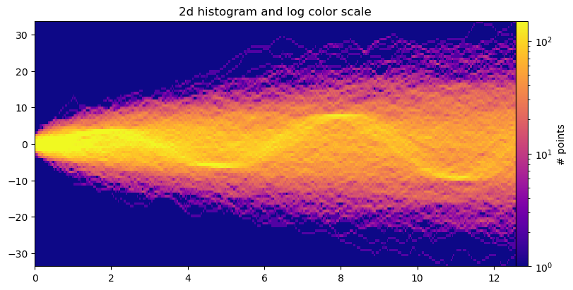
While we do assume that you have had some exposure to programming (at the level of CIS 1100), we do not assume that you’ve worked with Python before. This is not a programming class, and so our strategy will be to give you the minimum background necessary to solve cool problems. With that in mind, you’ll see that code blocks and their outputs, such as the one below, will be integrated throughout the course notes.

Even more exciting is that if you would like to experiment with this code, all you need to do is press the button below, and it will launch a fully editable and runnable version of this page that you can experiment with. Go ahead and give it a try!^[2]

from copy import copy

import numpy as np
import numpy.matlib
import matplotlib.pyplot as plt
from matplotlib.colors import LogNorm

# Make some data; a 1D random walk + small fraction of sine waves
num_series = 1000
num_points = 100
SNR = 0.10  # Signal to Noise Ratio
x = np.linspace(0, 4 * np.pi, num_points)
# Generate unbiased Gaussian random walks
Y = np.cumsum(np.random.randn(num_series, num_points), axis=-1)
# Generate sinusoidal signals
num_signal = int(round(SNR * num_series))
phi = (np.pi / 8) * np.random.randn(num_signal, 1)  # small random offset
Y[-num_signal:] = (
    np.sqrt(np.arange(num_points))[None, :]  # random walk RMS scaling factor
    * (np.sin(x[None, :] - phi)
       + 0.05 * np.random.randn(num_signal, num_points))  # small random noise
)


# Now we will convert the multiple time series into a histogram. Not only will
# the hidden signal be more visible, but it is also a much quicker procedure.
# Linearly interpolate between the points in each time series
num_fine = 800
x_fine = np.linspace(x.min(), x.max(), num_fine)
y_fine = np.empty((num_series, num_fine), dtype=float)
for i in range(num_series):
    y_fine[i, :] = np.interp(x_fine, x, Y[i, :])
y_fine = y_fine.flatten()
x_fine = np.matlib.repmat(x_fine, num_series, 1).flatten()

fig, axes = plt.subplots(figsize=(8, 4), constrained_layout=True)
cmap = copy(plt.cm.plasma)
cmap.set_bad(cmap(0))
h, xedges, yedges = np.histogram2d(x_fine, y_fine, bins=[400, 100])
pcm = axes.pcolormesh(xedges, yedges, h.T, cmap=cmap,
                         norm=LogNorm(vmax=1.5e2), rasterized=True)
fig.colorbar(pcm, ax=axes, label="# points", pad=0)
axes.set_title("2d histogram and log color scale");

Footnotes¶

By the way, did you try hovering over the equation number?
↩
Note that sometimes the code will look a little bit different in the notebook. That’s because we sometimes hide code that’s just needed for setup in the main notes.
↩

ESE 2030 - Linear Algebra with Applications to Engineering and AI

Tentative Schedule

Ch 1 Linear Algebraic Systems

1.1 Why Linear Systems?