1.1 Why Linear Systems?
They're everywhere!
Abstract
Our goal is to get to the good stuff quickly, and so we assume you have already seen things like matrices, vectors, and Gaussian Elimination in Math 1410. Our goal in this chapter is to remind you of what these things are, what they’re for, and how they can be automated and scaled out using computer code. We’ll see that with a little bit of work, we can already start asking really interesting questions, and solving some really interesting problems from science, engineering, and economics!
1Reading
Material related to this chapter, as well as additional exercises, can be found in LAA Ch. 1, ALA Ch. 1, and ILA Ch. 1.
2Learning Objectives
By the end of this chapter, you should know:
- how to solve small systems of linear equations by hand using Gaussian Elimination
- the basic concepts of scalar, vector, and matrix
- the fundamentals of matrix arithmetic
- how to compute inverses of small (2 x 2) matrices by hand, and understand the role of matrix inverses in solving systems of linear equations
- how to solve large systems of linear equations by computing the LU decomposition of a matrix, and how this relates to forward elimination and back substitution
- how to implement all of the above in Python using the standard computing package
NumPy
3Motivation: Why Linear Systems?
At this point, you might be wondering why an entire semester is devoted to solving systems of linear equations: after all, the world isn’t linear, and already saw how works in high-school. What more to it could there be? Well here’s a dirty little secret that ``big science’’ doesn’t want you to know: we (as mathematicians and engineers) only really know how to deal with linear systems, and so a typical approach to solving pretty much anything is to take a complicated problem and hammer away at it until you’ve reduced things to solving systems of linear equations. Now, these systems of linear equations might be very high-dimensional (involving thousands, millions, or even billions of parameters), and it may not be obvious how to get them, but they’re there. A completely non-exhaustive list of where systems of linear equations appear include economics, internet search, computational fluid dynamics, circuits, and robot motion planning. We’ll see a few simplified examples of these applications next before diving into the technical meat of this lecture.
3.1Motivating Application 1: Robot Motion Planning
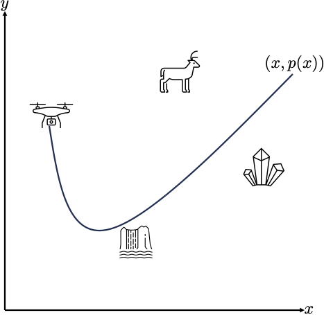
Suppose that I have quadcopter drone equipped with a camera, and I want to plan a path that brings my drone to three interesting things to photograph, for example, a waterfall, a cool rock, and a deer (for this example, we’ll assume the deer isn’t moving). We’ll assume that our drone is flying at the same elevation the whole time, meaning that its path evolves in the plane, as illustrated in Figure 1.
One approach to robot motion planning is to parameterize, that is describe, our drone’s path in terms of a function. Specifically, we can define our robots path as a function that ingests the current -position of our robot, and outputs the corresponding position as . For example, if we set , we are saying that our drone will follow a path that looks like a quadratic. Let’s stick with the quadratic parameterization for now, and think about how we might design , that is to say pick the parameters so that our drone’s path starts at our location, crosses the waterfall, cool rock, and then the deer. This problem is known as polynomial interpolation, because we’re trying to design a polynomial function (through our choice of ) that passes through, or interpolates between, a preset number of points. It turns out, this can be posed as a system of linear equations! We’ll revisit this example later in the lecture, see how it can be reduced to solving a system of linear equations. Later on in the class, we’ll answer questions like how many points can a quadratic motion plan interpolate, what is the ``best’’ path to pick if there are more than one that meet our requirements, and how to quickly construct new paths given an initial one.

Figure 1:Planning a path for a drone that passes through a prespecified set of points can be posed as solving a system of linear equations called an interpolation problem.
3.2Motivating Application 2: Network Flows
This example is adapted from p. 53 of LAA. Systems of linear equations arise naturally when scientists, engineers, or economists study the flow of some quantity through a network. For instance, urban planners and traffic engineers monitor the pattern of traffic flow in a grid of city streets. Electrical engineers calculate current flow through electrical circuits. Economists analyze the distribution of product from manufacturers to consumers through a network of wholesalers and retailers. Many modern networks lead to systems of equations involving hundreds, thousands, or even millions of variables and equations!
A network consists of a set of points called nodes with lines or arcs called edges that define connections between nodes. The direction of flow in each edge is indicated by an arrow, with positive flows in the direction of the arrow, and negative flows in the opposite direction. The flow amount or rate is either specified (via a number) or is denoted by a variable.
The basic assumption of network flow is that of conservation of flow, i.e., that the total flow into the network equals the total flow out of the network, and that the total flow into a node equals the total flout of the node. This has a very clear practical meaning depending on the application. For circuits, this is a restatement of Kirchoff’s current law. For traffic flow, this means that cars cannot spontaneously appear or disappear from the road. For distribution networks, this means that no product is lost (or created) while it is being transported.

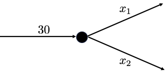
Figure 2:Flow conservation at a node can be written as a linear equation. Here, flow is conserved when .
For example, Figure 2 shows 30 units of flowing ino a node through one incoming edge, and two outgoing edges with flows and . For flow to be conserved here, we must have that . In a similar fashion, we can write down linear equations that balance the flow entering and leaving each node. The problem of network analysis is to determine the flow in each branch when only partial information (such as flow into and out of the network) is known.