1.9 Case Study: Modeling Network Flow using Systems of Linear Equations

1What is network flow?¶

Network flow models can be used to capture traffic flowing through a road network, water through a grid of pipes, or information flowing through the internet. In this section, we will use systems of linear equations to understand how to allocate flows (traffic, water, internet packets) across links (roads, pipes, network links) in order to meet demand (how much traffic must flow in and out of a network). We’ll also explore what happens when links are modified or deleted.

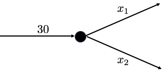
A key modeling assumption that we make is that flow is conserved, i.e., flows leaving a node have to equal flows leaving a node. Here we use the term node to describe where different links (roads, pipes, etc.) meet, i.e., nodes are where links intersect. In the figure below, flow conservation means that $x_1+x_2 = 30$ . This is a very reasonable assumption: for example, if we’re talking about road traffic, it means that all cars that enter a road network eventually leave it, and that no cars can spontaneously appear or disappear within the road network. Similarly, if we’re talking about internet traffic, it means that data can’t appear out of thin air, that all data entering the network eventually leaves it, and that packets can’t be dropped (this is not always true for internet traffic, but we definitely prefer it when no data is lost!).

2What Linear Algebra tools do we need to model network flow?¶

2.1Concepts¶

Gaussian Elimination / Row Reduction

2.2Computation¶

3Small Example¶

Let’s consider a system of pipes.

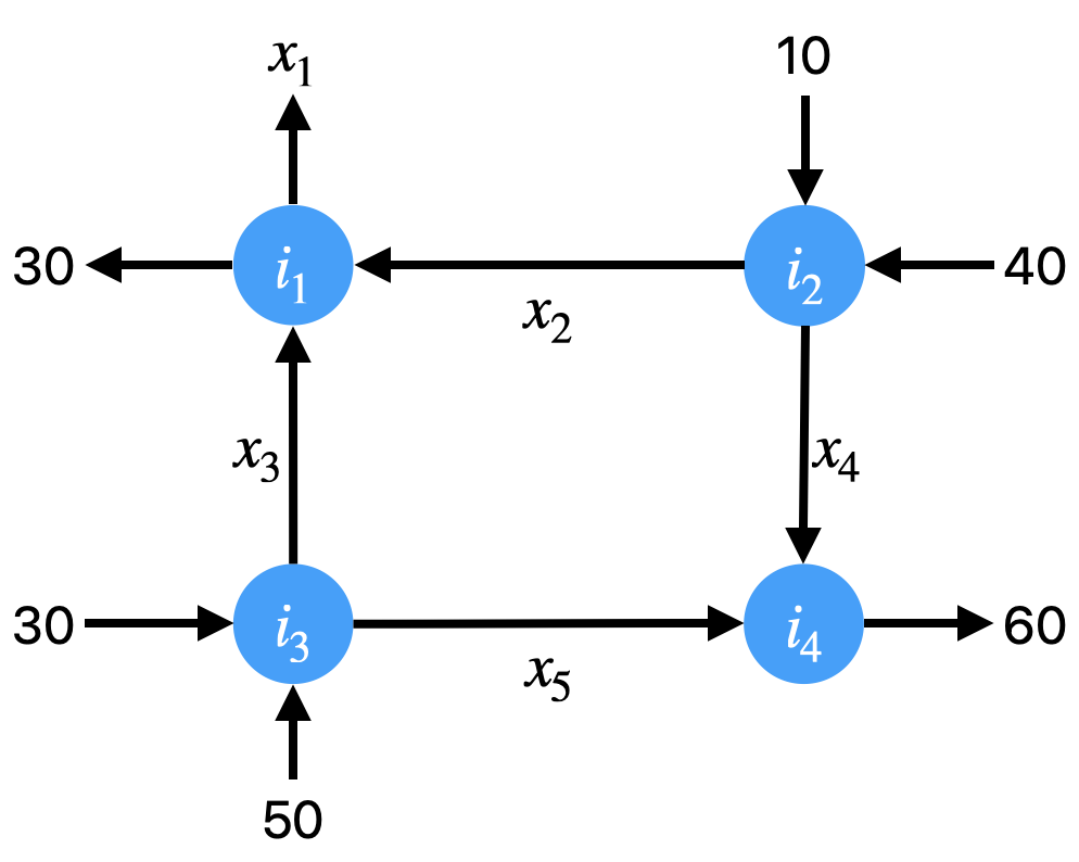
Because of our assumption that the total inflows and outflows are conserved, we can say that for each intersection $\text{inflow} - \text{outflow} = 0$ . We make our first observation: each intersection, or node, in the graph above leads to an equation. We can rearrange terms, and get the following equation, that $\text{inflow} = \text{outflow}$ . This is fairly intuitive, and we’ll use this law to create our system of equations. We also know that the total outflows leaving the system must be equal to the total inflows entering the system: we’ll call this total flow conservation.

\begin{align} \text{inflow} &= \text{outflow} \\ 10 + 40 + 30 + 50 &= 60 + 30 + x_1 &[\text{total conservation}] \\ x_2 + x_3 &= x_1 + 30 &[\text{from } i_1] \\ 10 + 40 &= x_2 + x_4 &[\text{from } i_2] \\ 30 + 50 &= x_3 + x_5 &[\text{from } i_3] \\ x_5 + x_4 &= 60 &[\text{from } i_4] \\ \end{align}

(1)

Each equation above represents an equality that results from our original assumption. The first equation shows the total conservation, and the next 4 lines show the equations for each intersection. Rearranging to have the unknowns $x_i$ on the left, and the knowns on the right, we get the following system of linear equations:

\begin{align} \text{inflow} &= \text{outflow} \\ 1x_1 + 0x_2 + 0x_3 + 0x_4 + 0x_5 &= 40 &[\text{total conservation}] \\ -1x_1 + 1x_2 + 1x_3 + 0x_4 + 0x_5 &= 30 &[\text{from } i_1] \\ 0x_1 + 1x_2 + 0x_3 + 1x_4 + 0x_5 &= 50 &[\text{from } i_2] \\ 0x_1 + 0x_2 + 1x_3 + 0x_4 + 1x_5 &= 80 &[\text{from } i_3] \\ 0x_1 + 0x_2 + 0x_3 + 1x_4 + 1x_5 &= 60 &[\text{from } i_4], \\ \end{align}

(2)

which we can put in $A\vv x = \vv b$ form:

\left[ \begin{array}{ccccc} %x_1 & x_2 &x_3 & x_4 &x_5\\\hline 1 & 0 & 0 & 0 & 0 \\ -1 & 1 & 1 & 0 & 0 \\ 0 & 1 & 0 & 1 & 0 \\ 0 & 0 & 1 & 0 & 1 \\ 0 & 0 & 0 & 1 & 1 \\ \end{array} \right] \left[ \begin{array}{c} x_1 \\ x_2 \\ x_3 \\ x_4 \\ x_5 \end{array} \right] = \left[ \begin{array}{cccccc} 40 \\ 30 \\ 50 \\ 80 \\ 60 \\ \end{array} \right]

(3)

We can construct the augmented matrix $[A | \vv b]$ for this system below:

\left[ \begin{array}{ccccc|c} & & A & & & \vv b\\\hline 1 & 0 & 0 & 0 & 0 & 40 \\ -1 & 1 & 1 & 0 & 0 & 30 \\ 0 & 1 & 0 & 1 & 0 & 50 \\ 0 & 0 & 1 & 0 & 1 & 80 \\ 0 & 0 & 0 & 1 & 1 & 60 \\ \end{array} \right]

(4)

4Python Implementation¶

We’ll work with SymPy to go through the steps of reducing the augmented matrix into row echelon form, and then solving for the general solutin.

import numpy as np
from numpy.linalg import solve
from sympy import Matrix, latex

augmented_matrix = np.array([
    [1 , 0 , 0 , 0,   0, 40],
    [-1 , 1 , 1 , 0 , 0, 30],
    [0 , 1 , 0 , 1, 0, 50],
    [0 , 0 , 1 , 0 , 1, 80],
    [0 , 0 , 0 , 1,   1, 60],
])
A = augmented_matrix[:,:-1]  # We take the first part of the augmented matrix, which represents A [: <- This means every row, :-1 <- This means all but the last column]
b = augmented_matrix[:, -1]  # Now the second part, which represents b [: <- This means every row, -1 <- This means only the last column]

matrix = Matrix(augmented_matrix)
matrix

Loading...

row_echelon_matrix = matrix.echelon_form(simplify=True)
row_echelon_matrix

Loading...

Placing this in equation form again, we get the below. There is no pivot in the 5th column, so $x_5$ is free.

\begin{align} 1x_1 + 0x_2 + 0x_3 + 0x_4 + 0x_5 &= 40 \\ 0x_1 + 1x_2 + 1x_3 + 0x_4 + 0x_5 &= 70 \\ 0x_1 + 0x_2 + -1x_3 + 1x_4 + 0x_5 &= -20 \\ 0x_1 + 0x_2 + 0x_3 + -1x_4 + -1x_5 &= -60 \\ \end{align}

(5)

Simplifying, we get the following system of equations:

\begin{align} x_1 &= 40 \\ x_2 + x_3 &= 70 \\ -x_3 + x_4 &= -20 \\ x_4 + x_5 &= 60 \\ \end{align}

(6)

We proceed from the bottom, and express the basic variables in terms of the free variable $x_5$ . To get an expression to start, we can simplify the last equation to

x_4 = 60 -x_5

(7)

Using back substitution, we can first substitute $x_4$ into our third equation, yielding

\begin{align*} x_3 - x_4 &= 20 \\ x_3 - (60 - x_5) &= 20 \\ x_3 &= 20 + 60 - x_5 \\ x_3 &= 80 - x_5 \end{align*}

(8)

Again substituting $x_3$ into the second equation, we get:

\begin{align*} x_2 + x_3 &= 70 \\ x_2 + 80 - x_5 &= 70 \\ x_2 &= x_5 - 10 \end{align*}

(9)

Gathering all of these equations, we get the general solution:

\begin{align} x_1 &= 40 \\ x_2 &= x_5 - 10 \\ x_3 &= 80 - x_5 \\ x_4 &= 60 - x_5 \\ x_5 &= \text{free} \end{align}

(10)

Now, we need to apply some human reasoning, namely that none of the traffic flow can be negative! The equality $x_2 = x_5 - 10$ tell us that $x_5$ must be at least 10 (otherwise $x_2$ would be negative!), and the equality $x_4 = 60 - x_5$ tells us that $x_5$ can be at most 60 (otherwise $x_4$ would be negative!).

With that in mind, we pick $x_5=30$ , which corresponds to putting 30 units of flow on $x_5$ , and get the following specific solution:

\begin{align} x_1 &= 40 \\ x_2 &= 20 \\ x_3 &= 50 \\ x_4 &= 30 \\ x_5 &= 30 \end{align}

(11)

Let’s check our solution in the original equation:

x = np.array([40, 20, 50, 30, 30])
print(A@x)
print(b)
A@x == b

[40 30 50 80 60]
[40 30 50 80 60]

array([ True, True, True, True, True])

We got a solution!

5Penn Engineering Road Network¶

We can apply the same sort of thinking to roads!

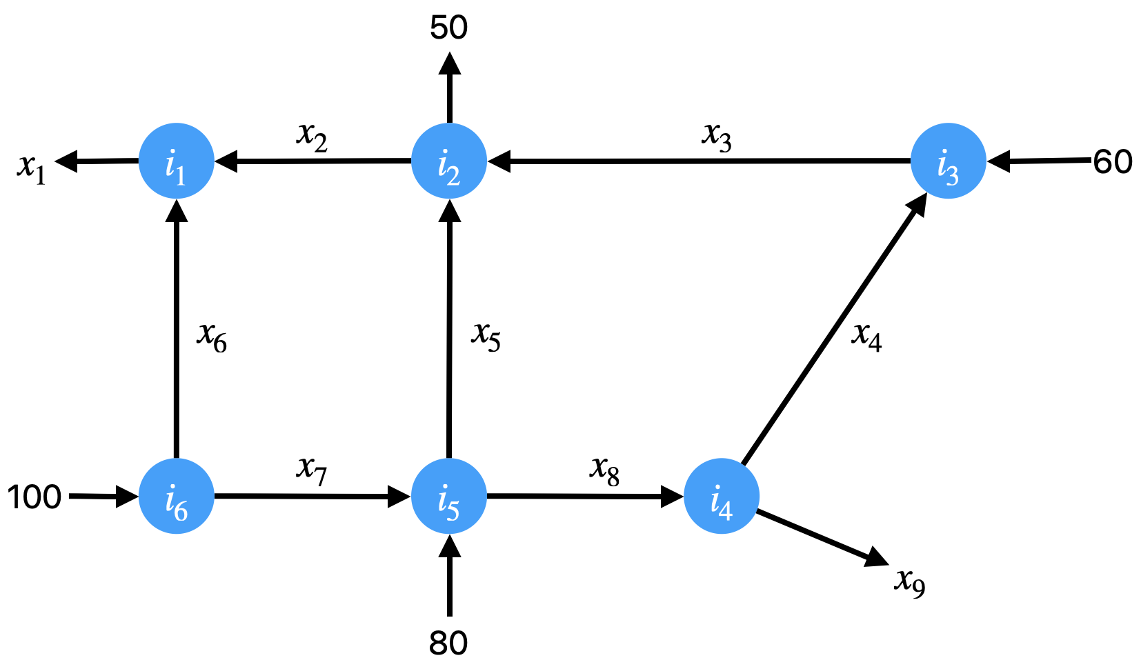
The above figure shows a road network that looks similar to that around Penn Engineering. We model these road networks the same way, by balancing the inflows and outflows of each node, and by enforcing total flow conservation as well. This yields the following system of linear equations:

\begin{align} \text{inflow} &= \text{outflow} \\ x_6 + x_2 &= x_1 &[\text{from } i_1]\\ x_3 + x_5 &= x_2 + 50 &[\text{from } i_2]\\ x_4 + 60 &= x_3 &[\text{from } i_3]\\ x_8 &= x_4 + x_9 &[\text{from } i_4]\\ 80 + x_7 &= x_{5} +x_8 &[\text{from } i_5]\\ 100 &= x_{6} + x_7 &[\text{from } i_6]\\ 100 + 80 + 60 &= x_1 + 50 + x_9 &[\text{total conservation}]\\ \end{align}

(12)

To put this in matrix form, we need to do the same as before, and reorganize terms.

\begin{align} \text{inflow} &= \text{outflow} \\ -x_1 + x_2 + x_6 &= 0 &[\text{from } i_1]\\ - x_2 + x_3 + x_5 &= 50 &[\text{from } i_2]\\ -x_3 + x_4 &= -60 &[\text{from } i_3]\\ x_4 - x_8 + x_9 &= 0 &[\text{from } i_4]\\ x_{5} -x_7 + x_8 &= 80 &[\text{from } i_5]\\ x_{6} + x_7 &= 100 &[\text{from } i_6]\\ x_1 + x_9 &= 190 &[\text{total conservation}]\\ \end{align}

(13)

This gives us the following augmented matrix

\left[ \begin{array}{ccccccccc|c} & & & & A & & & & & \vv b \\ \hline -1 & 1 & 0 & 0 & 0 & 1 & 0 & 0 & 0 & 0 \\ 0 & -1 & 1 & 0 & 1 & 0 & 0 & 0 & 0 & 50 \\ 0 & 0 & -1 & 1 & 0 & 0 & 0 & 0 & 0 & -60 \\ 0 & 0 & 0 & 1 & 0 & 0 & 0 & -1 & 1 & 0 \\ 0 & 0 & 0 & 0 & 1 & 0 & -1 & 1 & 0 & 80 \\ 0 & 0 & 0 & 0 & 0 & 1 & 1 & 0 & 0 & 100 \\ 1 & 0 & 0 & 0 & 0 & 0 & 0 & 0 & 1 & 190 \\ \end{array} \right] \begin{array}{l} \\ [\text{from } i_1]\\ [\text{from } i_2]\\ [\text{from } i_3]\\ [\text{from } i_4]\\ [\text{from } i_5]\\ [\text{from } i_6]\\ [\text{total conservation}]\\ \end{array}

(14)

augmented_matrix = np.array([
        [-1 , 1 , 0 , 0 , 0 , 1 , 0 , 0 , 0 , 0],
        [0 , -1 , 1 , 0 , 1 , 0 , 0 , 0 , 0 , 50],
        [0 , 0 , -1 , 1 , 0 , 0 , 0 , 0 , 0 , -60],
        [0 , 0 , 0 , 1 , 0 , 0 , 0 , -1 , 1 , 0],
        [0 , 0 , 0 , 0 , 1 , 0 , -1 , 1 , 0 , 80],
        [0 , 0 , 0 , 0 , 0 , 1 , 1 , 0 , 0 , 100],
        [1 , 0 , 0 , 0 , 0 , 0 , 0 , 0 , 1 , 190],
])
A = augmented_matrix[:,:-1]  # We take the first part of the augmented matrix, which represents A [: <- This means every row, :-1 <- This means all but the last column]
b = augmented_matrix[:, -1]  # Now the second part, which represents b [: <- This means every row, -1 <- This means only the last column]

matrix = Matrix(augmented_matrix)
echelon_form = matrix.echelon_form()
echelon_form

Loading...

Let’s print the row-echelon matrix in a nicer way:

\left[ \begin{array}{ccccccccc|c} & & & & U & & & & & \vv c \\ \hline -1 & 1 & 0 & 0 & 0 & 1 & 0 & 0 & 0 & 0\\ 0 & -1 & 1 & 0 & 1 & 0 & 0 & 0 & 0 & 50\\ 0 & 0 & -1 & 1 & 0 & 0 & 0 & 0 & 0 & -60\\ 0 & 0 & 0 & 1 & 0 & 0 & 0 & -1 & 1 & 0\\ 0 & 0 & 0 & 0 & 1 & 0 & -1 & 1 & 0 & 80\\ 0 & 0 & 0 & 0 & 0 & 1 & 1 & 0 & 0 & 100\\ 0 & 0 & 0 & 0 & 0 & 0 & 0 & 0 & 0 & 0 \end{array} \right]

(15)

Looking at the row-echelon form, we should notice a few things. First, that the last row is empty. Second, that there are not pivots in every column. In the columns for $x_7, x_{8}, x_{9}$ , there are no pivots. This means there are 3 free variables in this system. This makes sense, because we have only 6 intersections, giving 6 equations, but 9 flows, representing 9 variables. In order to find a solution, let’s set all of those free variables to be zero. We can think of this as closing all of the roads that are free variables.

Let’s solve for the free variables in terms of the basic variables:

First for $x_7$ :

\begin{align*} x_6 + x_7 &= 100 \\ x_7 &= 100 - x_6 \end{align*}

(16)

We know that if $x_7>100$ , then $x_6$ will be negative.

Now for $x_{8}$ :

\begin{align*} x_5 - x_7 + x_8 &= 80 \\ x_8 &= 80 - x_5 + x_7 \end{align*}

(17)

We also know that $x_8$ cannot be more than 80.

For $x_{9}$ :

\begin{align*} x_4 - x_8 + x_9 &= 0 \\ x_9 &= -x_4 + x_8 \end{align*}

(18)

Now let’s solve for the system, setting $x_7, x_8, x_9$ to be equal to 0. To do this, we first select all of the columns from the augmented matrix which correspond to basic variables.

smaller_augmented_matrix = np.array(echelon_form[:,[0,1,2,3,4,5,9]]).astype(np.float64)
"""
Above, we just selected all of the rows that correspond to the non-free variables. 
If the free variables are zero, then we can freely subtract them from the rest of the equations.
"""
# smaller_augmented_matrix = np.vstack([smaller_augmented_matrix, 
#                                       np.array([[0,0,0,0,0,0,0,0,1,0,80]]),
#                                      ])
smaller_augmented_matrix = smaller_augmented_matrix[:-1,:]
smaller_augmented_matrix

array([[ -1.,   1.,   0.,   0.,   0.,   1.,   0.],
       [  0.,  -1.,   1.,   0.,   1.,   0.,  50.],
       [  0.,   0.,  -1.,   1.,   0.,   0., -60.],
       [  0.,   0.,   0.,   1.,   0.,   0.,   0.],
       [  0.,   0.,   0.,   0.,   1.,   0.,  80.],
       [  0.,   0.,   0.,   0.,   0.,   1., 100.]])

Now that there are pivots in all columns, we can try to use numpy’s solve method to get a solution.

sA = smaller_augmented_matrix[:,:-1]  # We take the first part of the augmented matrix, which represents A [: <- This means every row, :-1 <- This means all but the last column]
sb = smaller_augmented_matrix[:, -1]  # Now the second part, which represents b [: <- This means every row, -1 <- This means only the last column]

x = solve(sA,sb)
x

array([190., 90., 60., 0., 80., 100.])

Let’s write these solutions down first.

\begin{align} x_1 &= 190 \\ x_2 &= 90 \\ x_3 &= 60 \\ x_4 &= 0 \\ x_5 &= 80 \\ x_6 &= 100 \\ \end{align}

(19)

One key thing to remember is that these variables are currently unconstrained. In our road network, a negative number means that traffic is flowing the wrong way. Let’s verify that the free variables we specified are actually zero, and see what we can learn from each solution.

\begin{align*} x_7 &= 100 - x_6 \\ x_7 &= 0 \end{align*}

(20)

\begin{align*} x_8 &= 80 - x_5 + x_7 \\ x_8 &= 80 - 80 + 0 \\ &= 0 \end{align*}

(21)

\begin{align*} x_9 &= -x_4 + x_8 \\ x_9 &= 0 + 0 \\ &= 0 \end{align*}

(22)

Now let’s check our solution:

x=\begin{bmatrix} x_1 \\ x_2 \\ x_3 \\ x_4 \\ x_5 \\ x_6 \\ x_7 \\ x_8 \\ x_9 \end{bmatrix} =\begin{bmatrix} 190 \\ 90 \\ 60 \\ 0 \\ 80 \\ 100 \\ 0 \\ 0 \\ 0 \end{bmatrix}

(23)

x = np.array([190,90,60,0,80,100,0,0,0])
print(A@x)
print(b)
print(A@x == b)

[  0  50 -60   0  80 100 190]
[  0  50 -60   0  80 100 190]
[ True  True  True  True  True  True  True]

As an extension, if you want to try to solve the same system, but fix the values for the free variables to different values. One way to do this would be to add equations to the system of equations that fix the values of specific variables. For example, you could add a row fixing $x_7 = 10$ like so:

\left[ \begin{array}{ccccccccc|c} x_1 & x_2 & x_3 & x_4 & x_5 & x_6 & x_7 & x_8 & x_9 & \vv c \\ \hline 0 & 0 & 0 & 0 & 0 & 0 & 1 & 0 & 0 & 10\\ \end{array} \right]

(24)

If you’re interested in modeling traffic flow, check out the Cellular Transmission Model and Networked Macroscopic Fundamental Diagram models for more info on how traffic flow is modeled in practice, and some approaches to control traffic lights.

1.9 Case Study: Modeling Network Flow using Systems of Linear Equations

1What is network flow?¶

2What Linear Algebra tools do we need to model network flow?¶

2.1Concepts¶

2.2Computation¶

3Small Example¶

4Python Implementation¶

5Penn Engineering Road Network¶

6Related Resources¶