8.4 Case Study: Implementing a Mini-Page-Rank

import numpy as np

1Learning objectives¶

In this case study, we will:

Walk through implementing the Page Rank algorithm on a toy internet
Understand through example its key mathematical design choices.

2Surfing a Toy Internet¶

Let’s first quickly review the motivation behind Page Rank. Page Rank, as developed by Google cofounders Sergey Brin and Larry Page, is an algorithm to produce an, at least in its original form, global relevance ranking of websites. As we’ve seen in lecture, the key idea is that by continuously clicking links and going to new webpages, one can model a user’s probability of landing at any given website as a random walk.

Mathematically, sufficiently “well-behaved” random walks, more specifically regular Markov Processes, are nice in that as one keeps iterating the transition matrix, the state vector converges to a fixed “steady-state vector”, implying that it doesn’t matter what webpage a user starts on initially, the long-run probability of visiting each website is the same. Of course, there are many pathologies that make these well-behaved Markov Processes a poor model of web usage, for example “dangling nodes”, where a link leads to a webpage that has not outgoing links. Avoiding these pathologies is what makes Page Rank more than just computing the top eigenvector of a transition matrix.

Let’s start by downloading a toy internet with a total of six indexed webpages.

# A helper function to download a file from a website
try:
    from urllib2 import urlopen
except ImportError:
    from urllib.request import urlopen

def progress_bar_downloader(url, fname, progress_update_every=5):
    #from http://stackoverflow.com/questions/22676/how-do-i-download-a-file-over-http-using-python/22776#22776
    u = urlopen(url)
    f = open(fname, 'wb')
    meta = u.info()
    file_size = int(meta.get("Content-Length"))
    print("Downloading: %s Bytes: %s" % (fname, file_size))
    file_size_dl = 0
    block_sz = 8192
    p = 0
    while True:
        buffer = u.read(block_sz)
        if not buffer:
            break
        file_size_dl += len(buffer)
        f.write(buffer)
        if (file_size_dl * 100. / file_size) > p:
            status = r"%10d  [%3.2f%%]" % (file_size_dl, file_size_dl * 100. / file_size)
            print(status)
            p += progress_update_every
    f.close()

# Download a 6-page miniweb from a ubc course
import os

pages_link = 'http://www.cs.ubc.ca/~nando/340-2009/lectures/pages.zip'
dlname = 'pages.zip'
#This will unzip into a directory called pages
if not os.path.exists('./%s' % dlname):
    progress_bar_downloader(pages_link, dlname)
    os.system('unzip %s' % dlname)
else:
    print('%s already downloaded!' % dlname)

pages.zip already downloaded!

Our website is now comprised of the following pages: “angelinajolie.html”, “bradpitt.html”, “jenniferaniston.html”, “jonvoight.html”, “martinscorcese.html”, and “robertdeniro.html”.

Some sample webpages look like:

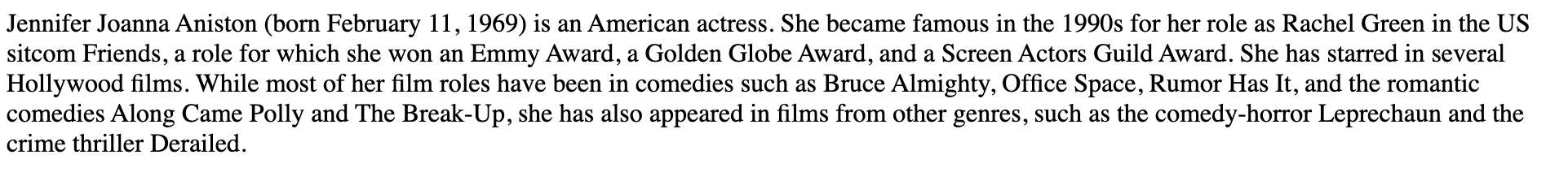
As we can see, these webpages contain various number of links to the other webpages in our small internet. Now we can trawl through and collect the links leaving each webpage.

3Building the Matrix¶

To build the link matrix, we parse websites for outgoing links. For every page referenced by a page, we will add a 1 to the associated row. Adding a small term eps to all entries, in order guarantee the matrix is fully connected and renormalizing will ensure a valid link matrix with a unique solution.

#Quick and dirty link parsing as per http://www.cs.ubc.ca/~nando/540b-2011/lectures/book540.pdf
links = {}
for fname in os.listdir(dlname[:-4]):
    links[fname] = []
    f = open(dlname[:-4] + '/' + fname)
    for line in f.readlines():
        while True:
            p = line.partition('<a href="http://')[2]
            if p == '':
                break
            url, _, line = p.partition('\">')
            links[fname].append(url)
    f.close()

for key in links.keys():
    print(f"Links in {key}: {links[key]}")

Links in robertdeniro.html: ['martinscorcese.html']
Links in jenniferaniston.html: []
Links in martinscorcese.html: []
Links in jonvoight.html: ['angelinajolie.html', 'angelinajolie.html', 'bradpitt.html']
Links in angelinajolie.html: ['jonvoight.html', 'bradpitt.html']
Links in bradpitt.html: ['jenniferaniston.html', 'angelinajolie.html', 'martinscorcese.html', 'angelinajolie.html']

Graphically, our little internet looks like:

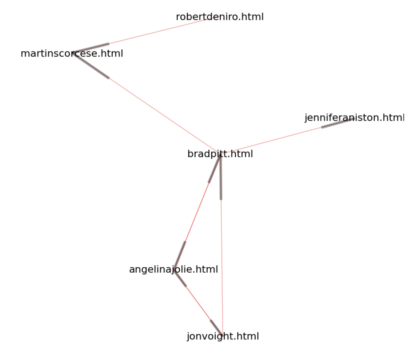
internet graph — A visual of the toy internet. Black bars indicate a link going in to a webpage.

To form a transition matrix associated with this (directed) graph, recall that the basic form of Page Rank assumes that when a web surfer is on a given page, they will click on any link with equal probability. With this assumption in mind, we can go through the link dictionary we formed just now and create the transition matrix in numpy.

num_pages = len(links.keys())
P = np.zeros((num_pages, num_pages))

#Assign identity numbers to each page, along with a reverse lookup
idx = {}
lookup = {}
for n,k in enumerate(sorted(links.keys())):
    idx[k] = n
    lookup[n] = k

#Go through all keys, and add a 1 for each link to another page
for k in links.keys():
    v = links[k]
    for e in v:
        P[idx[e],idx[k]] += 1
    if len(v) > 0:
        P[:, idx[k]] = P[:, idx[k]]/np.sum(P[:, idx[k]])
    else:
        # no outgoing links: user stays at current state
        P[idx[k], idx[k]] = 1

print('Raw transition matrix P\n', P)

Raw transition matrix P
 [[0.         0.5        0.         0.66666667 0.         0.        ]
 [0.5        0.         0.         0.33333333 0.         0.        ]
 [0.         0.25       1.         0.         0.         0.        ]
 [0.5        0.         0.         0.         0.         0.        ]
 [0.         0.25       0.         0.         1.         1.        ]
 [0.         0.         0.         0.         0.         0.        ]]

Unfortunately, there are some columns in the transition that are all 0 apart from the diagonal entry, corresponding to webpages that have no outgoing links. This implies that the transition matrix in its current form is not a regular transition matrix. To see why this is problematic, consider a web-user starting on page 3, i.e. $\bold x(1) = \bm 0 & 0 & 1 & 0 & 0 & 0 \em^\top$ . Since there are no outgoing links, the next state vector will be $\bold x(2) = \bold x(1)$ , ensuring that it remains at $\bold x(1)$ for all time. Similarly, since there are incoming links to these dead-end webpages, iterating the transition matrix will shift more and more weight from other webpages that have outgoing links to the dead-end links.

Not only is this behavior undesirable--we don’t want to put undue weight on websites just because they have no outgoing links--this also implies that the long-run $\bold x(k)$ becomes dependent on the initial distribution. For example, starting at page 3 will have $\bold x(k) = \bm 0 & 0 & 1 & 0 & 0 & 0 \em^\top$ for all $k$ , whereas starting at page 5 will have $\bold x(k) = \bm 0 & 0 & 0 & 0 & 1 & 0 \em^\top$ for all $k$ .

x = np.array([0,0,1,0,0,0])
print("x(1) = Px =", P@x)
print("x(2) = P^2 x =", P@P@x)

x = np.ones(6)/6
print("\nInit x:", np.round(x,3))
for i in range(50):
    # print("next x:", G@x)
    x = P@x
    # print("Sum of entries:",np.sum(x))
print("x(50) =", np.round(x,3))

x = np.array([0.1, 0.1, 0.5, 0., 0.2, 0.1])
print("\nInit x:", np.round(x,3) )
for i in range(50):
    # print("next x:", G@x)
    x = P@x
    # print("Sum of entries:",np.sum(x))
print("x(50) =", np.round(x,3))

x(1) = Px = [0. 0. 1. 0. 0. 0.]
x(2) = P^2 x = [0. 0. 1. 0. 0. 0.]

Init x: [0.167 0.167 0.167 0.167 0.167 0.167]
x(50) = [0.    0.    0.417 0.    0.583 0.   ]

Init x: [0.1 0.1 0.5 0.  0.2 0.1]
x(50) = [0.  0.  0.6 0.  0.4 0. ]

To summarize, naively computing the transition matrix is not sufficient for Page-Rank because:

Dead-end webpages (“dangling nodes”) get unnaturally weighted due to not having outgoing links.
The ranking, i.e. sorted entries of the converged state vector, is therefore not unique.

This motivates the first adjustment Page rank proposes:

Therefore, once a user reaches a dead-end, instead of staying there with 100% probability (which is an extremely poor model of reality anyways), Page Rank instead assumes the user resets and starts over at a completely random website. Of course, this random website is in practice not chosen uniformly at random across every single website out there, and the Page Rank Google used in production certainly did many proprietary optimizations upon this, but this adjustment suffices for our basic model.

Is this adjustment enough? What happens when there are cycles? For example, let us consider a $4 \times 4$ transition matrix (with no dangling nodes!):

\begin{align*} P = \bm 0.5 & 0.5 & 0 & 0 \\ 0.5 & 0.5 & 0 & 0 \\ 0 & 0 & 0.5 & 0.5 \\ 0 & 0 & 0.5 & 0.5 \em. \end{align*}

(1)

Notice there are no entries that cross between $1,2$ and $3,4$ . Therefore, if the user starts on page 1 or 2, they will stay there perpetually, and similarly if they start on page 3 or 4. This also implies there is no unique long-run state probability vector, since $\bold x(k)$ is once again dependent on the initial $\bold x(1)$ .

P0 = np.array([[0.5, 0.5, 0, 0],[0.5, 0.5, 0, 0],[0, 0, 0.5, 0.5],[0, 0, 0.5, 0.5]])
print("P = ", P0)
x = np.array([1, 0, 0, 0])
print("\nInit x:", np.round(x,3) )
for i in range(50):
    # print("next x:", G@x)
    x = P0@x
    # print("Sum of entries:",np.sum(x))
print("x(50) =", np.round(x,3))

x = np.array([0, 0, 1, 0])
print("\nInit x:", np.round(x,3) )
for i in range(50):
    # print("next x:", G@x)
    x = P0@x
    # print("Sum of entries:",np.sum(x))
print("x(50) =", np.round(x,3))

P =  [[0.5 0.5 0.  0. ]
 [0.5 0.5 0.  0. ]
 [0.  0.  0.5 0.5]
 [0.  0.  0.5 0.5]]

Init x: [1 0 0 0]
x(50) = [0.5 0.5 0.  0. ]

Init x: [0 0 1 0]
x(50) = [0.  0.  0.5 0.5]

This pathology is in spirit the same as dangling nodes. Instead of dangling nodes, there may now be dangling sets of nodes that only link within each other. Therefore, an additional adjustment needs to be made to ensure these dangling communities do not occur, which brings us to the second adjustment.

As discussed in lecture, this amounts to taking a weighted sum between the transition matrix and a matrix $K = [k_{ij}] \in \R^{n \times n}$ where $k_{ij} = 1/n$ for all $i,j$ .

G = pP + (1-p)K,

(2)

This all depends on the weighting parameter $p \in (0,1)$ , which discussed in class was approximately 0.85 in practice.

G = np.zeros((num_pages, num_pages))
for k in links.keys():
    v = links[k]
    for e in v:
        G[idx[e],idx[k]] += 1
    if len(v) > 0:
        G[:, idx[k]] = G[:, idx[k]]/np.sum(G[:, idx[k]])
    else:
        # no outgoing links: user stays at current state
        G[idx[k], idx[k]] = 1
        
eps = 1. / num_pages
p = 0.85
G = p * G + (1-p)*eps * np.ones((num_pages, num_pages))
print('Processed link matrix G guaranteeing unique solution\n', G)

Processed link matrix G guaranteeing unique solution
 [[0.025      0.45       0.025      0.59166667 0.025      0.025     ]
 [0.45       0.025      0.025      0.30833333 0.025      0.025     ]
 [0.025      0.2375     0.875      0.025      0.025      0.025     ]
 [0.45       0.025      0.025      0.025      0.025      0.025     ]
 [0.025      0.2375     0.025      0.025      0.875      0.875     ]
 [0.025      0.025      0.025      0.025      0.025      0.025     ]]

This matrix $G$ should now permit a unique $x^\star$ such that $x^\star = G x^\star$ . To sanity check this, we can list the eigenvalues of $G$ . If $x^\star$ is unique, then the multiplicity of the eigenvalue $\lambda = 1$ should be 1 (why?). Let’s check this using np.linalg.eigvals:

G_eigs = np.linalg.eigvals(G)
P_eigs = np.linalg.eigvals(P)

print("Eigs of G:", np.round(np.sort(G_eigs)[::-1],3))
print("Eigs of original P:", np.round(np.sort(P_eigs)[::-1],3))

Eigs of G: [ 1.     0.85   0.703 -0.    -0.126 -0.577]
Eigs of original P: [ 1.     1.     0.827  0.    -0.148 -0.679]

Therefore, we see that $G$ does indeed ensure a unique long-run $x^\star$ , whereas the original transition matrix does not. To solve for the corresponding $x^\star$ that satisfies $x^\star = G x^\star$ , we could just use np.linalg.eig to directly compute it. However, we note that this can be posed as a regression problem.

\begin{align*} &x^\star = G x^\star \\ \implies\;& (I-G)x^\star = \boldsymbol 0. \end{align*}

(3)

The unique non-zero solution to the above problem is precisely $x^\star$ . However, we have to ensure the least-squares solver doesn’t just default to the trivial solution $(I-G)\boldsymbol 0 = \boldsymbol 0$ . A trick to avoid this is to augment the left and right hand sides of the equation. Define $A := I-G$ . Then consider the augmented system formed by adding a row of 1s to $A$ and a last entry of 1 to the right-hand side.

\begin{align*} \bm &A & \\ 1 & \cdots & 1 \em \bold x^\star = \bm \boldsymbol 0 \\ 1 \em. \end{align*}

(4)

One can verify that $\bold x^\star$ solving the original system also solves this system. Additionally, since this system is now “tall” a.k.a. overdetermined, the solution is guaranteed to be unique!

# In order to eliminate the trivial solution, we append the constraint
# that sum(x) == 1
ones = np.ones(shape=(1,num_pages))
e_7 = np.zeros(shape=(num_pages+1,))
e_7[-1] = 1
Gg = np.vstack((np.eye(num_pages)-G,ones))
print('Augmented matrix with sum constraint\n', Gg)

Augmented matrix with sum constraint
 [[ 0.975      -0.45       -0.025      -0.59166667 -0.025      -0.025     ]
 [-0.45        0.975      -0.025      -0.30833333 -0.025      -0.025     ]
 [-0.025      -0.2375      0.125      -0.025      -0.025      -0.025     ]
 [-0.45       -0.025      -0.025       0.975      -0.025      -0.025     ]
 [-0.025      -0.2375     -0.025      -0.025       0.125      -0.875     ]
 [-0.025      -0.025      -0.025      -0.025      -0.025       0.975     ]
 [ 1.          1.          1.          1.          1.          1.        ]]

p_solve, residuals, _, _ = np.linalg.lstsq(Gg, e_7, rcond=None)

# We verify that the residual is zero
assert np.abs(residuals)<10e-12, f'Something went wrong, we have nonzero residual: {residual}'

We have therefore passed all the checks to output a unique page-rank vector. Let’s check it out.

print('Our importance rankings are ', p_solve)
print('Our page rankings, from least to most important, are therefore ', np.argsort(p_solve))
print('This is the mapping between the indices and pages: \n', idx)

Our importance rankings are  [0.10012444 0.08669287 0.28948157 0.06755289 0.43114823 0.025     ]
Our page rankings, from least to most important, are therefore  [5 3 1 0 2 4]
This is the mapping between the indices and pages: 
 {'angelinajolie.html': 0, 'bradpitt.html': 1, 'jenniferaniston.html': 2, 'jonvoight.html': 3, 'martinscorcese.html': 4, 'robertdeniro.html': 5}

4Wait, where does Search come into this?¶

Having put quite some attention on Page Rank, one might be wondering: we’ve output a vector that measures the global relevance of websites on the internet. That’s great, but where does Google’s claim-to-fame Search come in? A global ranking doesn’t seem to have any effect on returning personalized rankings relevant to a search query.

This is where years of hyperoptimization and billions of dollars on Google’s part comes in, but we can in fact build a primitive search engine without too much effort. A naive idea is the following:

Break down a search query to its component words
Restrict attention only webpages containing the component words
Return webpage therein with highest Page Rank score.

5Now let’s search¶

Now that the PageRank for each page is calculated, how can we actually perform a search? Note that this is pure programming/parsing, and not related to class content, but may still be of interest to you.

We create an index of every word in a page. When we search for words, we will then sort the output by the PageRank of those pages, thus ordering the links by the importance we associated with that page.

search = {}
for fname in os.listdir(dlname[:-4]):
    f = open(dlname[:-4] + '/' + fname)
    for line in f.readlines():
        #Ignore header lines
        if '<' in line or '>' in line:
            continue
        words = line.strip().split(' ')
        words = filter(lambda x: x != '', words)
        #Remove references like [1], [2]
        words = filter(lambda x: not ('[' in x or ']' in x), words)

    for word in words:
        if word in search:
            if fname in search[word]:
                search[word][fname] += 1
            else:
                search[word][fname] = 1
        else:
            search[word] = {fname: 1}
    f.close()

Our search engine is not very sophisticated, taking only individual words, and we can only search for queries found within search.keys()--case must also match.

print(search.keys())
print("\n")
print("Some values from search dict:\n", list(search.values())[0:50])

dict_keys(['Robert', 'Mario', 'De', 'Niro,', 'Jr.', '(born', 'August', '17,', '1943)', 'is', 'an', 'American', 'actor,', 'director,', 'and', 'producer.', 'She', 'has', 'starred', 'in', 'several', 'Hollywood', 'films.', 'While', 'most', 'of', 'her', 'film', 'roles', 'have', 'been', 'comedies', 'such', 'as', 'Bruce', 'Almighty,', 'Office', 'Space,', 'Rumor', 'Has', 'It,', 'the', 'romantic', 'Along', 'Came', 'Polly', 'The', 'Break-Up,', 'she', 'also', 'appeared', 'films', 'from', 'other', 'genres,', 'comedy-horror', 'Leprechaun', 'crime', 'thriller', 'Derailed.', "Scorsese's", 'body', 'work', 'addresses', 'themes', 'Italian', 'identity,', 'Roman', 'Catholic', 'concepts', 'guilt', 'machismo,', 'violence.', 'Scorsese', 'widely', 'considered', 'to', 'be', 'one', 'significant', 'influential', 'filmmakers', 'his', 'era,', 'directing', 'landmark', 'Taxi', 'Driver,', 'Raging', 'Bull', 'Goodfellas;', 'all', 'which', 'he', 'collaborated', 'on', 'with', 'actor', 'He', 'earned', 'Academy', 'Award', 'for', 'Best', 'Director', 'Departed', 'MFA', 'New', 'York', 'University', 'Tisch', 'School', 'Arts.', 'Jonathan', 'Vincent', '"Jon"', 'Voight', 'December', '29,', '1938)', 'television', 'actor.', 'had', 'a', 'long', 'distinguished', 'career', 'both', 'leading', 'man', 'and,', 'recent', 'years,', 'character', 'extensive', 'compelling', 'range.', 'came', 'prominence', 'at', 'end', '1960s,', 'performance', 'would-be', 'hustler', "1969's", 'Picture', 'winner,', 'Midnight', 'Cowboy,', 'first', 'nomination.', 'Throughout', 'following', 'decades,', 'built', 'reputation', 'array', 'challenging', 'Deliverance', '(1972),', 'Coming', 'Home', '(1978),', 'received', 'Actor.', "Voight's", 'impersonation', 'sportscaster/journalist', 'Howard', 'Cosell,', '2001', 'biopic', 'Ali,', 'critical', 'raves', 'fourth', 'Oscar', 'seventh', 'season', '24', 'villain', 'Jonas', 'Hodges.', 'Angelina', 'Jolie', 'Voight;', 'June', '4,', '1975)', 'actress', 'Goodwill', 'Ambassador', 'UN', 'Refugee', 'Agency.', 'three', 'Golden', 'Globe', 'Awards,', 'two', 'Screen', 'Actors', 'Guild', 'Award.', 'promoted', 'humanitarian', 'causes', 'throughout', 'world,', 'noted', 'refugees', 'through', 'UNHCR.', 'cited', "world's", 'beautiful', 'women', 'off-screen', 'life', 'Pitt', 'began', 'acting', 'guest', 'appearances,', 'included', 'role', 'CBS', 'soap', 'opera', 'Dallas', '1987.', 'gained', 'recognition', 'cowboy', 'hitchhiker', 'who', 'seduces', 'Geena', "Davis's", '1991', 'road', 'movie', 'Thelma', '&', 'Louise.', "Pitt's", 'big-budget', 'productions', 'A', 'River', 'Runs', 'Through', 'It', '(1992)', 'Interview', 'Vampire', '(1994).', 'was', 'cast', 'opposite', 'Anthony', 'Hopkins', '1994', 'drama', 'Legends', 'Fall,', 'him', 'In', '1995,', 'gave', 'critically', 'acclaimed', 'performances', 'Seven', 'science', 'fiction', 'Twelve', 'Monkeys,', 'latter', 'earning', 'Supporting', 'Actor', 'Four', 'years', 'later', '1999,', 'cult', 'hit', 'Fight', 'Club.', 'Subsequently', '2001,', 'major', 'international', "Ocean's", 'Eleven', 'its', 'sequels', '(2004)', 'Thirteen', '(2007).', 'biggest', 'commercial', 'successes', 'Troy', 'Mr.', 'Mrs.', 'Smith', '(2005).', 'second', 'nomination', 'title', '2008', 'Curious', 'Case', 'Benjamin', 'Button.'])


Some values from search dict:
 [{'robertdeniro.html': 1, 'martinscorcese.html': 1}, {'robertdeniro.html': 1}, {'robertdeniro.html': 1, 'martinscorcese.html': 1}, {'robertdeniro.html': 1}, {'robertdeniro.html': 1}, {'robertdeniro.html': 1, 'jonvoight.html': 1, 'angelinajolie.html': 1}, {'robertdeniro.html': 1}, {'robertdeniro.html': 1}, {'robertdeniro.html': 1}, {'robertdeniro.html': 1, 'martinscorcese.html': 1, 'jonvoight.html': 1, 'angelinajolie.html': 3}, {'robertdeniro.html': 1, 'martinscorcese.html': 1, 'jonvoight.html': 4, 'angelinajolie.html': 2, 'bradpitt.html': 1}, {'robertdeniro.html': 1, 'martinscorcese.html': 2, 'jonvoight.html': 1, 'angelinajolie.html': 1}, {'robertdeniro.html': 1, 'jonvoight.html': 1}, {'robertdeniro.html': 1}, {'robertdeniro.html': 1, 'jenniferaniston.html': 3, 'martinscorcese.html': 5, 'jonvoight.html': 6, 'angelinajolie.html': 4, 'bradpitt.html': 6}, {'robertdeniro.html': 1}, {'jenniferaniston.html': 1, 'angelinajolie.html': 2}, {'jenniferaniston.html': 2, 'jonvoight.html': 3, 'angelinajolie.html': 3, 'bradpitt.html': 1}, {'jenniferaniston.html': 1, 'jonvoight.html': 1, 'bradpitt.html': 2}, {'jenniferaniston.html': 3, 'martinscorcese.html': 1, 'jonvoight.html': 5, 'bradpitt.html': 11}, {'jenniferaniston.html': 1}, {'jenniferaniston.html': 1}, {'jenniferaniston.html': 1}, {'jenniferaniston.html': 1}, {'jenniferaniston.html': 1, 'martinscorcese.html': 1, 'angelinajolie.html': 1}, {'jenniferaniston.html': 1, 'martinscorcese.html': 6, 'jonvoight.html': 4, 'angelinajolie.html': 1, 'bradpitt.html': 2}, {'jenniferaniston.html': 1, 'angelinajolie.html': 2}, {'jenniferaniston.html': 1, 'martinscorcese.html': 1, 'jonvoight.html': 1, 'bradpitt.html': 2}, {'jenniferaniston.html': 1, 'jonvoight.html': 1, 'bradpitt.html': 1}, {'jenniferaniston.html': 1}, {'jenniferaniston.html': 1, 'angelinajolie.html': 1}, {'jenniferaniston.html': 2}, {'jenniferaniston.html': 2, 'martinscorcese.html': 2, 'jonvoight.html': 1}, {'jenniferaniston.html': 2, 'martinscorcese.html': 2, 'jonvoight.html': 4, 'angelinajolie.html': 1, 'bradpitt.html': 1}, {'jenniferaniston.html': 1}, {'jenniferaniston.html': 1}, {'jenniferaniston.html': 1}, {'jenniferaniston.html': 1}, {'jenniferaniston.html': 1}, {'jenniferaniston.html': 1}, {'jenniferaniston.html': 1}, {'jenniferaniston.html': 3, 'martinscorcese.html': 4, 'jonvoight.html': 6, 'angelinajolie.html': 3, 'bradpitt.html': 13}, {'jenniferaniston.html': 1}, {'jenniferaniston.html': 1}, {'jenniferaniston.html': 1}, {'jenniferaniston.html': 1}, {'jenniferaniston.html': 1, 'martinscorcese.html': 1, 'bradpitt.html': 1}, {'jenniferaniston.html': 1}, {'jenniferaniston.html': 1}, {'jenniferaniston.html': 1}]

Therefore, inputting a search term into search[] will return the websites containing the term, from which we can the return the page with the highest Page Rank score.

6Ranking The Results¶

With words indexed, we can now complete the task. Searching for a particular word (in this case, ‘film’), we get back all the pages with references and counts. Sorting these so that the highest pagerank comes first, we see the Googley(TM) result for our tiny web.

def get_pr(fname):
    print(f'page: {fname}, pagerank: {p_solve[idx[fname]]}')
    return p_solve[idx[fname]]

r = search['films']
print(f"Pages containing 'films': {r}\n")

print("Associated Page Rank scores")

print("Sorted:", sorted(r, reverse=True, key=get_pr))

Pages containing 'films': {'jenniferaniston.html': 1, 'martinscorcese.html': 1, 'jonvoight.html': 1}

Associated Page Rank scores
page: jenniferaniston.html, pagerank: 0.28948156780637474
page: martinscorcese.html, pagerank: 0.4311482344730417
page: jonvoight.html, pagerank: 0.06755288679953375
Sorted: ['martinscorcese.html', 'jenniferaniston.html', 'jonvoight.html']

7Concluding remarks¶

We’ve now seen a prototype to Google’s Page Rank algorithm, as well as the various pathologies that motivated its various components. However, many parts of the algorithm we described leave many facets underexplored. For example, people certainly don’t reset to a completely random website, and will usually default to well-known domains like Wikipedia or Reddit. Also, how does one incorporate semantic meaning when considering search queries (Case Study 3.3 perhaps)? As food for thought, now knowing the idea behind Page Rank, come up with a few ideas of how Page Rank can be be exploited. This is a prelude to the decades-long Search Engine Optimization (SEO) saga.

Ch 8 Iteration

8.3 Page Rank and the Google Matrix

Ch 9 Symmetric Matrices

9.1 Eigenvalues of Symmetric Matrices