9.1 Eigenvalues of Symmetric Matrices

1Reading¶

Material related to this page, as well as additional exercises, can be found in ALA 8.5.

2Learning Objectives¶

By the end of this page, you should know:

the properties of eigenvalues and eigenvectors of symmetric matrices
the Spectral theorem
the geometric interpretation of a linear transformation when the matrix is symmetric

3Symmetric Matrix¶

A square matrix $A$ is said to be symmetric if $A = A^T$ . For example, all 2×2 symmetric and 3×3 symmetric matrices are of the form:

\begin{bmatrix} a & b \\ b & c \end{bmatrix} \quad \text{and} \quad \begin{bmatrix} a & b & c \\ b & d & e \\ c & e & f \end{bmatrix}

(1)

Symmetric matrices arise in many practical contexts: an important one we will spend time on next lecture are covariance matrices. For now, we simply take them as a family of interesting matrices.

Symmetric matrices enjoy many interesting properties, including the following one which will be the focus of this lecture:

We’ll spend the rest of this lecture exploring the consequences of this remarkable theorem, before diving into applications over the next few lectures.

First, we work through a few simple examples to see this theorem in action.

Example 1

$A = \begin{bmatrix} 3 & 1 \\ 1 & 3 \end{bmatrix}$ . We’ve seen this matrix in previous examples. It has eigenvalues $\lambda_1 = 4$ and $\lambda_2 = 2$ with corresponding eigenvectors $\vv v_1 = (1,1)$ and $\vv v_2 = (-1,1)$ . We easily verify that $\vv v_1^T \vv v_2 = 0$ , and hence are orthogonal. We construct an orthonormal basis by dividing each eigenvector by its Euclidean norm:

\vv u_1 = \frac{\vv v_1}{\|\vv v_1\|} = \frac{1}{\sqrt{2}} \begin{bmatrix} 1 \\ 1 \end{bmatrix} \quad \text{and} \quad \vv u_2 = \frac{\vv v_2}{\|\vv v_2\|} = \frac{1}{\sqrt{2}} \begin{bmatrix} -1 \\ 1 \end{bmatrix}

(2)

Example 2

Consider the symmetric matrix $A = \begin{bmatrix} 5 & -4 & 2 \\ -4 & 5 & 2 \\ 2 & 2 & -1 \end{bmatrix}$ . Computing the eigenvalues/eigenvectors of $A$ (e.g., using np.linalg.eig) we see that

\lambda_1 = 9, \vv v_1 = \begin{bmatrix} 1 \\ -1 \\ 0 \end{bmatrix}, \quad \lambda_2 = 3, \vv v_2 = \begin{bmatrix} 1 \\ 1 \\ 1 \end{bmatrix}, \quad \text{and} \quad \lambda_3 = -3, \vv v_3 = \begin{bmatrix} 1 \\ 1 \\ -2 \end{bmatrix}.

(3)

You can check that these vectors are pairwise orthogonal: $\vv v_i^T \vv v_j = 0$ for $i \neq j$ , and hence form an orthogonal basis for $\mathbb{R}^3$ . An orthonormal basis is obtained by the corresponding unit norm eigenvectors:

\vv u_1 = \frac{1}{\sqrt{2}} \begin{bmatrix} -1 \\ 1 \\ 0 \end{bmatrix}, \quad \vv u_2 = \frac{1}{\sqrt{3}} \begin{bmatrix} 1 \\ 1 \\ 1 \end{bmatrix}, \quad \text{and} \quad \vv u_3 = \frac{1}{\sqrt{6}} \begin{bmatrix} 1 \\ 1 \\ -2 \end{bmatrix}.

(4)

4The Spectral Theorem¶

The theorem above tells us that every real, symmetric matrix admits an eigenvector basis, and hence is diagonalizable. Furthermore, we can always choose eigenvectors that form an orthonormal basis—hence, the diagonalizing matrix takes a particularly simple form.

Remember that a matrix $Q \in \mathbb{R}^{n \times n}$ is orthogonal if and only if its columns form an orthonormal basis of $\mathbb{R}^n$ . Alternatively, we can characterize orthogonal matrices by the condition that $Q^T Q = Q Q^T = I$ , i.e., $Q^{-1} = Q^T$ .

If we use this orthonormal eigenbasis when diagonalizing a symmetric matrix $A$ , we obtain its spectral factorization:

5Geometric Interpretation¶

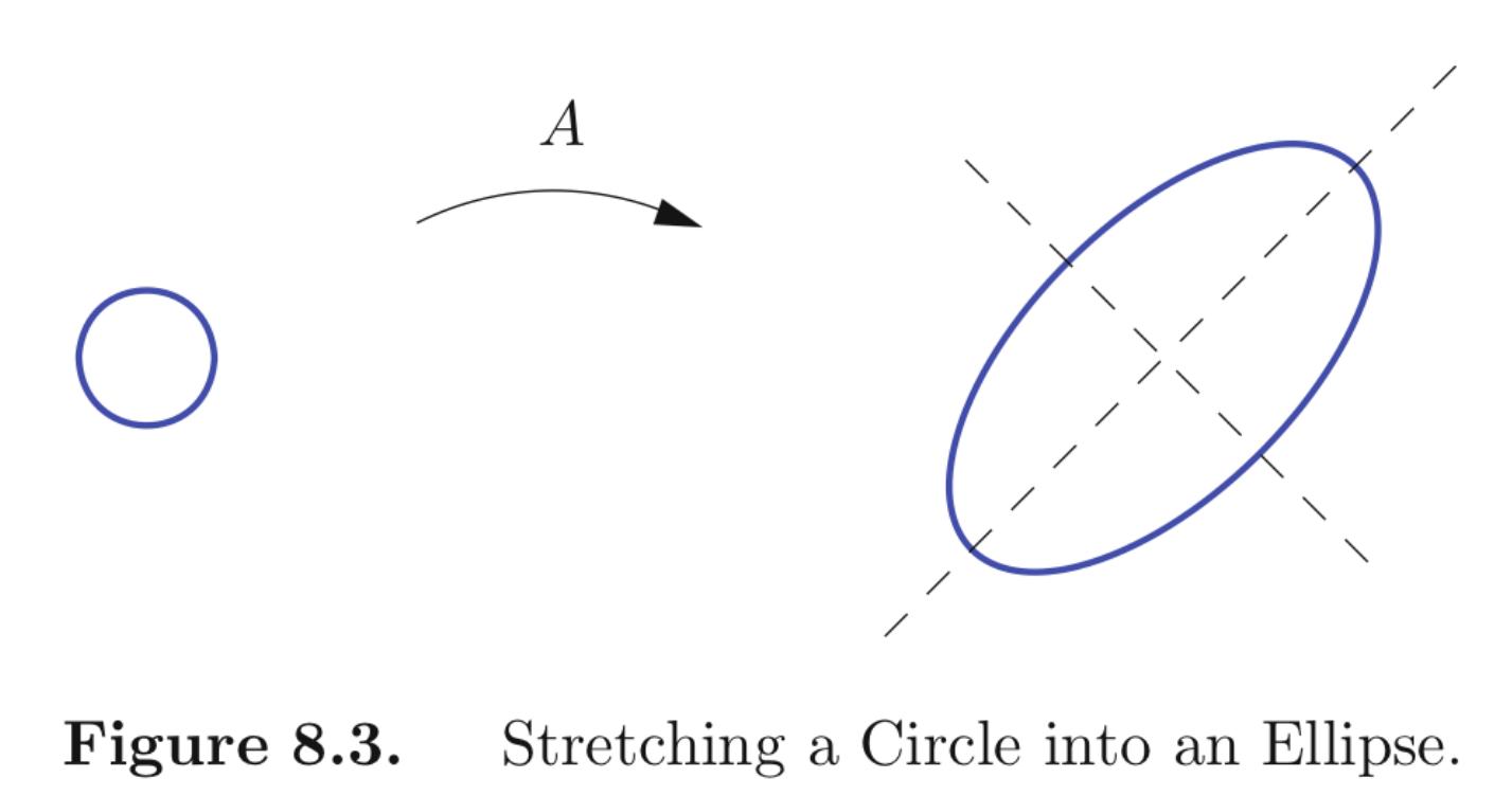
You can always choose $Q$ to have $\det Q = 1$ ; such a $Q$ represents a rotation. Thus the diagonalization of a symmetric matrix can be interpreted as a rotation of the coordinate system so that the orthogonal eigenvectors align with the coordinate axes. Therefore, the linear transformation $L(\vv x) = A\vv x$ for which $A$ has all positive eigenvalues can be interpreted as a combination of stretches in $n$ mutually orthogonal directions. One way to visualize this is to consider what $L(\vv x)$ does to the unit Euclidean sphere $S = \{ \vv x \in \mathbb{R}^n \mid \|\vv x\| = 1\}$ : stretching it in orthogonal directions will transform it into an ellipsoid : $E = L(S) = \{ A\vv x \mid \|\vv x\| = 1\}$ whose principal axes are the directions of stretch, i.e., the eigenvectors of $A$ .