9.2 Quadratic Forms & Positive Definite Matrices

1Reading¶

Material related to this page, as well as additional exercises, can be found in ALA 3.4 and LAA 7.2.

2Learning Objectives¶

By the end of this page, you should know:

what are quadratic forms
the geometry of quadratic forms and what are level sets
the different classes of quadratic forms
how a quadratic form relates to the corresponding positive definite matrix and its eigen values

3Defining Quadratic Forms¶

One common place where symmetric matrices arise in application is in defining quadratic forms, which pop up in engineering design (in design criteria and optimization), signal processing (as output noise power), physics (as potential & kinetic energy), differential geometry (as normal curvature of surfaces), economics (as utility functions), and statistics (in confidence ellipsoids).

where $K = K^T \in \mathbb{R}^{n \times n}$ is an $n \times n$ symmetric matrix. Such quadratic forms arise frequently in applications of linear algebra. For example, setting $K = I_n$ and $\vv z = A \vv x - \vv b$ , we recover the least-squares objective

q(A\vv x-\vv b) = (A\vv x-\vv b)^T(A \vv x-\vv b) = \|A\vv x-\vv b\|^2.

(2)

Example 1

For $\vv x \in \mathbb{R}^3$ , let $q(\vv x) = 5x_1^2 + 3x_2^2 + 2x_3^2 - x_1x_2 + 8x_2x_3$ . Find a matrix $K = K^T \in \mathbb{R}^{3\times3}$ such that $q(\vv x) = \vv x^T k \vv x$ .

The approach is to recognize that the coefficients of $x_1^2$ , $x_2^2$ , and $x_3^2$ go on the diagonal of $K$ . To make $K$ symmetric, the coefficients for $x_ix_j$ , $i\neq j$ , should be evenly split between the $(i,j)$ and $(j,i)$ entries of $L$ .

Using this strategy, we obtain:

q(\vv x) = \vv x^T k \vv x = \begin{bmatrix} x_1 \\ x_2 \\ x_3 \end{bmatrix}^T \begin{bmatrix} 5 & -\frac{1}{2} & 0 \\ -\frac{1}{2} & 3 & 4 \\ 0 & 4 & 2 \end{bmatrix} \begin{bmatrix} x_1 \\ x_2 \\ x_3 \end{bmatrix}.

(3)

4The Geometry of Quadratic Forms¶

We’ll focus on understanding the geometry of quadratic forms on $\mathbb{R}^{2 \times 2}$ . Let $K = K^T \in \mathbb{R}^{2\times 2}$ be an invertible $2\times 2$ symmetric matrix, and let’s consider quadratic forms:

q(\vv x) = \begin{bmatrix} x_1 \\ x_2 \end{bmatrix}^T \begin{bmatrix} k_{11} & k_{12} \\ k_{12} & k_{22} \end{bmatrix} \begin{bmatrix} x_1 \\ x_2 \end{bmatrix} = k_{11}x_1^2 + 2k_{12}x_1x_2 + k_{22}x_2^2 \qquad (\text{2D}).

(4)

What kinds of functions do these define? We study this question by looking at the level sets of $q(\vv x)$ .

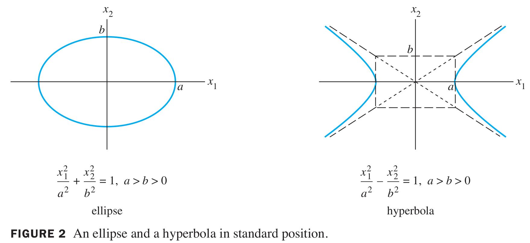
It is possible to show that such level sets correspond to either an ellipse, a hyperbola, two intersecting lines, a single point, or no points at all. If $K$ is a diagonal matrix, the graph of (5) is in standard position, as seen below:

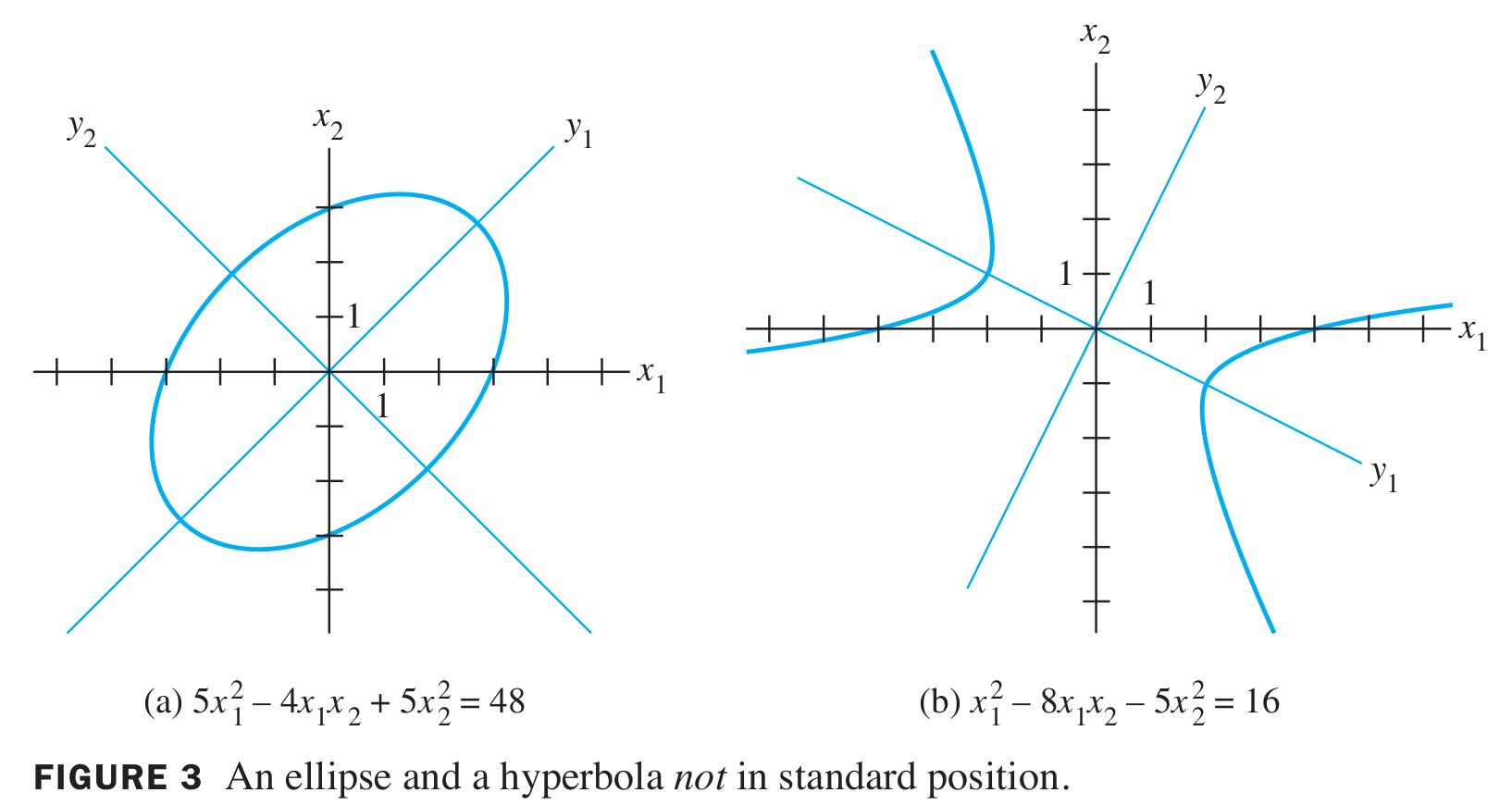
If $K$ is not diagonal, the graph of (5) is rotated out of standard position, as shown below:

The principle axes of these rotated graphs are defined by the eigenvectors of $K$ , and amount to a new coordinate system (or change of basis) with respect to which the graph is in standard position.

Example 2

The ellipse in Figure 2 is the graph of equation $5x_1^2 - 4x_1x_2 + 5x_2^2 = 48$ . This is given by the quadratic form

q(\vv x) = \vv x^T K \vv x = \begin{bmatrix} x_1 \\ x_2 \end{bmatrix}^T \begin{bmatrix} 5 & -2 \\ -2 & 5 \end{bmatrix} \begin{bmatrix} x_1 \\ x_2 \end{bmatrix}.

(6)

The eigenvalues/vectors of $K$ are:

\lambda_1 = 3, \quad \vv v_1 = \begin{bmatrix} 1 \\ 1 \end{bmatrix} \quad \text{and} \quad \lambda_2 = 7, \quad \vv v_2 = \begin{bmatrix} -1 \\ 1 \end{bmatrix}.

(7)

We define the orthonormal basis: $\vv u_1 = \frac{\vv v_1}{\|\vv v_1\|} = \begin{bmatrix} \frac{1}{\sqrt{2}} \\ \frac{1}{\sqrt{2}} \end{bmatrix}$ and $\vv u_2 = \frac{\vv v_2}{\|\vv v_2\|} = \begin{bmatrix} -\frac{1}{\sqrt{2}} \\ \frac{1}{\sqrt{2}} \end{bmatrix}$

and set $Q = \bm \vv u_1 & \vv u_2\em = \frac{1}{\sqrt{2}} \begin{bmatrix} 1 & -1 \\ 1 & 1 \end{bmatrix}$ . Then $q(\vv x) = \vv x^T Q \Lambda Q^T \vv x$ , and the change of variables $\vv y = Q^T \vv x$ produces the quadratic form

q(\vv y) = \vv y^T \Lambda \vv y = 3y_1^2 + 7y_2^2.

(8)

These axes are shown in the ellipse of Figure 2 (labeled $y_1$ and $y_2$ ).

5Classifying Quadratic Forms¶

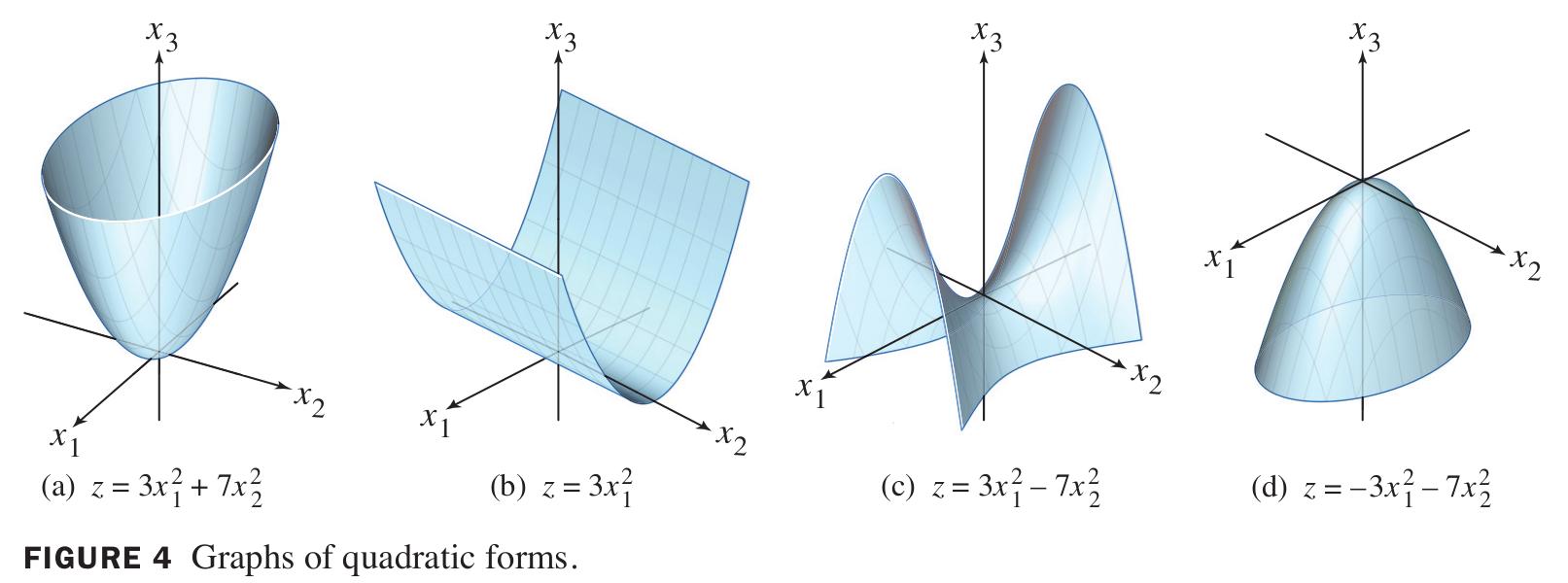
Depending on the eigenvalues of the symmetric matrix $K$ defining a quadratic form $q(\vv x) = \vv x^T K \vv x$ , the resulting function can look very different. The figure below shows four different quadratic forms plotted as functions with domain $\mathbb{R}^2$ , i.e., we are plotting $(x, y, q(x,y))$ .

Notice that except for $\vv x = 0$ , the values $q(\vv x)$ are all positive in Fig. 4(a) and all negative in Fig. 4(d). If we take horizontal cross-sections of these plots, we get an ellipse (these are the level sets $C_{\alpha}$ we saw earlier!), the vertical cross-sections of Fig. 4(c) are hyperbolas.

This simple $2 \times 2$ example illustrates the following definitions.

Also, $q(\vv x)$ is said to be positive (negative) semidefinite if $q(\vv x) \geq 0$ ( $\leq 0$ ) $\forall \vv x$ : in particular, we now allow $q(\vv x) = 0$ for nonzero $\vv x$ .

The following theorem leverages the spectral factorization of a symmetric matrix to characterize quadratic forms in terms of the eigenvalues of $K$ .

Theorem 1

Let $K = K^T \in \mathbb{R}^{n \times n}$ be a symmetric $n \times n$ matrix. Then a quadratic form is

positive definite if and only if all eigenvalues of $K$ are positive,
negative definite if and only if all eigenvalues of $K$ are negative,
indefinite if and only if $K$ has both positive and negative eigenvalues.

Proof 1 (Proof of Theorem 1)

Let $K = Q \Lambda Q^T$ be the spectral factorization of $K$ : $Q$ has columns defining an orthonormal eigenbasis for $\mathbb{R}^n$ and $\Lambda = \text{diag}(\lambda_1, \ldots, \lambda_n)$ is a diagonal matrix of eigenvalues of $K$ . Then:

\begin{align*} q(\vv x) &= \vv x^T k \vv x = \vv x^T Q \Lambda Q^T \vv x &= ( Q^T \vv x)^T \Lambda (Q^T \vv x) = \vv y^T \Lambda \vv y, \quad \text{where} \ \vv y = Q^{\top} \vv x \\ &= \lambda_1 y_1^2 + \cdots + \lambda_n y_n^2. \end{align*}

(9)

Since $Q$ is orthogonal, there is a one-to-one correspondence between all nonzero $\vv x$ and nonzero $\vv y$ ( $\vv y = Q^T \vv x$ , $\vv x = Q\vv y$ ).

Thus, the values of $q(\vv x)$ for $\vv x \neq 0$ coincide with the values of (9): the sign of $q(\vv x)$ is therefore controlled by the signs of the eigenvalues $\lambda_1, \ldots, \lambda_n$ as described in the theorem.