4.5 Least Squares - ESE 2030 📏

1Reading¶

Material related to this page, as well as additional exercises, can be found in LAA 6.5 and VMLS 12.1.

2Learning Objectives¶

By the end of this page, you should know:

the least squares problem and how to solve it
how the least squares problem relates to a solving an approximate linear system

3Introduction: Inconsistent Linear Equations¶

Suppose we are presented with an inconsistent set of linear equations $A \vv x \approx \vv b$ . This typically coincides with $A \in \mathbb{R}^{m \times n}$ being a “tall matrix”, i.e., $m > n$ . This corresponds to an overdetermined system of $m$ linear equations in $n$ unknowns. A typical setup assumes this arises is one of data fitting: we are given feature variables $\vv a_i \in \mathbb{R}^n$ and response variables ${b_i \in \mathbb{R}}$ , and we believe that $\vv a_i^{\top} \vv x \approx b_i$ for measurements $i=1,\ldots, m$ and $\vv x \in \mathbb{R}^n$ are our model parameters. We will revisit this application in detail later.

The question then becomes, if no $\vv x \in \mathbb{R}^n$ exists such that $A \vv x = \vv b$ exists, what should we do? A natural idea is to select an $\vv x$ that makes the error or residual $\vv r = A\vv x - \vv b$ as small as possible, i.e., to find the $\vv x$ that minimizes $\|\vv r\| = \|A\vv x - \vv b\|$ . Now minimizing the residual or its square gives the same answer, so we may as well minimize

\|A\vv x - \vv b\|^2 = \|\vv r\|^2 = r_1^2 + \cdots + r_m^2,

(1)

the sum of squares of the residuals.

4The Least Squares Problem¶

4.1Solving by Orthogonal Projection¶

There are many ways of deriving the solution to (LS): you may have seen a vector calculus-based derivation in Math 1410. Here, we will use our new understanding of orthogonal projections to provide an intuitive and elegant geometric derivation.

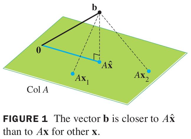
Our starting point is a column interpretation of the least squares objective: let $\vv a_1, \ldots, \vv a_n \in \mathbb{R}^m$ be the columns of $A$ : then the least squares (LS) problem is the problem of finding a linear combination of the columns that is closest to the vector $\vv b \in \mathbb{R}^m$ , with coefficients specified by $\vv x$ :

\|A\vv x - \vv b\|^2 = \|(x_1a_1 + \cdots + x_na_n) - b\|^2

(3)

To prove the above geometrically intuitive fact (see Figure 1), we need to decompose $\vv b$ into its orthogonal projection onto Col $(A)$ , which we denote by $\hat{\vv b}$ , and the element in its orthogonal complement Col $(A)$ , which we denote by $\vv e$ . Recall $\vv b, \hat{\vv b}, \vv e\in \mathbb{R}^m$ and Col $(A) \subset \mathbb{R}^m$ .

We then have that

\vv r = A \vv x - \vv b = \left(A \vv x - \hat{\vv b}\right) - \vv e.

(4)

Since $A \vv x, \hat{\vv b} \in$ Col $(A)$ , so is $A \vv x - \hat{\vv b}$ (why?), and thus we have decomposed $\vv r$ into components lying in Col $(A)$ and Col $(A)^{\perp}$ . Using our generalized Pythagorean theorem, it then follows that

\|A \vv x - \vv b\|^2 = \|\vv r\|^2 = \|A \vv x - \hat{\vv b}\|^2 + \|\vv e\|^2.

(5)

The above expression can be made as small as possible be choosing $\hat{\vv x}$ such that $A\hat{\vv x} = \hat{\vv b}$ , which always has a solution (why?) leaving the residual error $\|\vv e\|^2 = \|\vv b - \hat{\vv b}\|^2$ , ie, the component of $\vv b$ that is orthogonal to Col $(A)$ .

This gives us a nice geometric interpretation of the lest squares solution $\hat{\vv x}$ , but how should we compute it? We now recall from here that Col $(A)^{\perp} =$ Null $(A^{\top})$ . So, we therefore have that $\vv e \in$ Null $(A^{\top})$ . This means that

A^{\top} \vv e=A^{\top} \left(\vv b - \hat{\vv b}\right) = A^{\top} \left(\vv b - A \hat{\vv x}\right) = 0.

(6)

or, equivalently that

A^{\top} A \hat{\vv x} = A^{\top} \vv b. \ (\textrm{NE})

(7)

The above equations are the normal equations associated with the lest squares problem specified by $A$ and $\vv b$ . We have just informally argued that the set of least squares solutions $\hat{\vv x}$ coincide with the set of solutions to the normal equations (NE): this is in fact true, and can be proven (we wont do that here).

Thus, we have reduced solving a least squares problem to our favorite problem, solving a system of linear equations! One question you might have is when do the normal equations (NE) have a unique solution? The answer, perhaps unsurprisingly, is when the columns of are linearly independent, and hence form a basis for Col $(A)$ . The following theorem is a useful summary of our discussion thus fur:

Example 1

Consider the linear system

\begin{align*} x_1 + 2x_2 &= 1, \\ 3x_1 - x_2 + x_3 &= 0, \\ -x_1 + 2x_2 + x_3 &= -1, \\ x_1 - x_2 - 2x_3 &= 2, \\ 2x_1 + x_2 - x_3 &= 2. \end{align*}

(9)

consisting of 5 equations in 3 unknowns. The coeﬃcient matrix and right-hand side are

A = \bm 1 & 2 & 0 \\ 3 & -1 & 1 \\ -1 & 2 & 1 \\ 1 & -1 & -2 \\ 2 & 1 & -1 \em, \quad \mathbf{b} = \bm 1 \\ 0 \\ -1 \\ 2 \\ 2 \em

(10)

A direct application of Gaussian Elimination shows that $\vv{b}\notin$ Col $A$ , and so the system is incompatible — it has no solution. Of course, to apply the least squares method, we are not required to check this in advance. If the system has a solution, it is the least squares solution too, and the least squares method will ﬁnd it.

Let us ﬁnd the least squares solution based on the Euclidean norm, uisng the XLS formula.

K = A^T A = \bm 16 & -2 & -2 \\ -2 & 11 & 2 \\ -2 & 2 & 7 \em, \quad \mathbf{f} = A^T \mathbf{b} = \bm 8 \\ 0 \\ -7 \em

(11)

Solving the $3 \times 3$ system of normal equations $K \vv x = \vv f$ by Gaussian Elimination, we ﬁnd

\mathbf{x}^* = K^{-1}\mathbf{f} \approx \bm .4119 & .2482 & -.9532 \em^T

(12)

to be the least squares solution to the system. The least squares error is

\|\mathbf{b} - A\mathbf{x}^*\|^2 \approx \| \bm -.0917, .0342, .1313, .0701, .0252 \em ^T\|^2 \approx .03236.

(13)

which is reasonably small — indicating that the system is, roughly speaking, not too incompatible.

An alternative strategy is to begin by orthonormalizing the columns of $A$ using Gram– Schmidt. We can then apply the orthogonal projection formula to construct the same least squares solution. We suggest you to try this strategy as an exercise.

Exercise 1

Find a least-squares solution of the inconsistent system $A\mathbf{x} = \mathbf{b}$ for

A = \begin{bmatrix} 4 & 0 \\ 0 & 2 \\ 1 & 1 \end{bmatrix}, \quad \mathbf{b} = \begin{bmatrix} 2 \\ 0 \\ 11 \end{bmatrix}

(14)

Solution to Exercise 1

To use normal equations (NE), compute:

A^TA = \begin{bmatrix} 4 & 0 & 1 \\ 0 & 2 & 1 \end{bmatrix} \begin{bmatrix} 4 & 0 \\ 0 & 2 \\ 1 & 1 \end{bmatrix} = \begin{bmatrix} 17 & 1 \\ 1 & 5 \end{bmatrix}

(15)

A^T\mathbf{b} = \begin{bmatrix} 4 & 0 & 1 \\ 0 & 2 & 1 \end{bmatrix} \begin{bmatrix} 2 \\ 0 \\ 11 \end{bmatrix} = \begin{bmatrix} 19 \\ 11 \end{bmatrix}

(16)

Then the equation $A^TA\mathbf{x} = A^T\mathbf{b}$ becomes

\begin{bmatrix} 17 & 1 \\ 1 & 5 \end{bmatrix} \begin{bmatrix} x_1 \\ x_2 \end{bmatrix} = \begin{bmatrix} 19 \\ 11 \end{bmatrix}

(17)

Row operations can be used to solve this system, but since $A^TA$ is invertible and $2 \times 2$ , it is probably faster to compute

(A^TA)^{-1} = \frac{1}{84} \begin{bmatrix} 5 & -1 \\ -1 & 17 \end{bmatrix}

(18)

and then to solve $A^TA\mathbf{x} = A^T\mathbf{b}$ as

\begin{align*} \bar{\mathbf{x}} &= (A^TA)^{-1}A^T\mathbf{b} \\ &= \frac{1}{84} \begin{bmatrix} 5 & -1 \\ -1 & 17 \end{bmatrix} \begin{bmatrix} 19 \\ 11 \end{bmatrix} = \frac{1}{84} \begin{bmatrix} 84 \\ 168 \end{bmatrix} = \begin{bmatrix} 1 \\ 2 \end{bmatrix} \end{align*}

(19)

Exercise 2

Find a least-squares solution of $A\mathbf{x} = \mathbf{b}$ for

A = \begin{bmatrix} 1 & 1 & 0 & 0 \\ 1 & 1 & 0 & 0 \\ 1 & 0 & 1 & 0 \\ 1 & 0 & 1 & 0 \\ 1 & 0 & 0 & 1 \\ 1 & 0 & 0 & 1 \end{bmatrix}, \quad \mathbf{b} = \begin{bmatrix} -3 \\ -1 \\ 0 \\ 2 \\ 5 \\ 1 \end{bmatrix}

(20)

Solution to Exercise 2

Compute

A^TA = \begin{bmatrix} 1 & 1 & 1 & 1 & 1 & 1 \\ 1 & 1 & 0 & 0 & 0 & 0 \\ 0 & 0 & 1 & 1 & 0 & 0 \\ 0 & 0 & 0 & 0 & 1 & 1 \end{bmatrix} \begin{bmatrix} 1 & 1 & 0 & 0 \\ 1 & 1 & 0 & 0 \\ 1 & 0 & 1 & 0 \\ 1 & 0 & 1 & 0 \\ 1 & 0 & 0 & 1 \\ 1 & 0 & 0 & 1 \end{bmatrix} = \begin{bmatrix} 6 & 2 & 2 & 2 \\ 2 & 2 & 0 & 0 \\ 2 & 0 & 2 & 0 \\ 2 & 0 & 0 & 2 \end{bmatrix}

(21)

A^T\mathbf{b} = \begin{bmatrix} 1 & 1 & 1 & 1 & 1 & 1 \\ 1 & 1 & 0 & 0 & 0 & 0 \\ 0 & 0 & 1 & 1 & 0 & 0 \\ 0 & 0 & 0 & 0 & 1 & 1 \end{bmatrix} \begin{bmatrix} -3 \\ -1 \\ 0 \\ 2 \\ 5 \\ 1 \end{bmatrix} = \begin{bmatrix} 4 \\ -4 \\ 2 \\ 6 \end{bmatrix}

(22)

The augmented matrix for $A^TA\mathbf{x} = A^T\mathbf{b}$ is

\begin{bmatrix} 6 & 2 & 2 & 2 & 4 \\ 2 & 2 & 0 & 0 & -4 \\ 2 & 0 & 2 & 0 & 2 \\ 2 & 0 & 0 & 2 & 6 \end{bmatrix} \sim \begin{bmatrix} 1 & 0 & 0 & 1 & 3 \\ 0 & 1 & 0 & -1 & -5 \\ 0 & 0 & 1 & -1 & -2 \\ 0 & 0 & 0 & 0 & 0 \end{bmatrix}

(23)

The general solution is $x_1 = 3 - x_4$ , $x_2 = -5 + x_4$ , $x_3 = -2 + x_4$ , and $x_4$ is free. So the general least-squares solution of $A\mathbf{x} = \mathbf{b}$ has the form

\hat{\mathbf{x}} = \begin{bmatrix} 3 \\ -5 \\ -2 \\ 0 \end{bmatrix} + x_4 \begin{bmatrix} -1 \\ 1 \\ 1 \\ 1 \end{bmatrix}

(24)

Exercise 3

Given $A$ and $\mathbf{b}$ as in Exercise 1, determine the least-squares error in the least-squares solution of $A\mathbf{x} = \mathbf{b}$ .

Solution to Exercise 3

From Exercise 1,

\mathbf{b} = \begin{bmatrix} 2 \\ 0 \\ 11 \end{bmatrix} \quad \text{and} \quad A\hat{\mathbf{x}} = \begin{bmatrix} 4 & 0 \\ 0 & 2 \\ 1 & 1 \end{bmatrix} \begin{bmatrix} 1 \\ 2 \end{bmatrix} = \begin{bmatrix} 4 \\ 4 \\ 3 \end{bmatrix}

(25)

Hence

\mathbf{b} - A\hat{\mathbf{x}} = \begin{bmatrix} 2 \\ 0 \\ 11 \end{bmatrix} - \begin{bmatrix} 4 \\ 4 \\ 3 \end{bmatrix} = \begin{bmatrix} -2 \\ -4 \\ 8 \end{bmatrix}

(26)

and

\|\mathbf{b} - A\hat{\mathbf{x}}\| = \sqrt{(-2)^2 + (-4)^2 + 8^2} = \sqrt{84}

(27)

The least-squares error is $\sqrt{84}$ . For any $\mathbf{x}$ in $\mathbb{R}^2$ , the distance between $\mathbf{b}$ and the vector $A\mathbf{x}$ is at least $\sqrt{84}$ . See Figure 2. Note that the least-squares solution $\hat{\mathbf{x}}$ itself does not appear in the figure.

Exercise 4

Find a least-squares solution of $A\mathbf{x} = \mathbf{b}$ for

A = \begin{bmatrix} 1 & -2 \\ 5 & 3 \end{bmatrix}, \quad \mathbf{b} = \begin{bmatrix} 8 \\ 1 \end{bmatrix}

(28)

Solution to Exercise 4

Compute

A^TA = \begin{bmatrix} 26 & 13 \\ 13 & 13 \end{bmatrix}

(29)

A^T\mathbf{b} = \begin{bmatrix} 1 & 5 \\ -2 & 3 \end{bmatrix} \begin{bmatrix} 8 \\ 1 \end{bmatrix} = \begin{bmatrix} 13 \\ -13 \end{bmatrix}

(30)

The augmented matrix for $A^TA\mathbf{x} = A^T\mathbf{b}$ is

\begin{bmatrix} 26 & 13 & 13 \\ 13 & 13 & -13 \end{bmatrix} \sim \begin{bmatrix} 26 & 13 & 13 \\ 0 & 6.5 & -19.5 \end{bmatrix}

(31)

Using backsubstitution, the solution to the above system is $x_2 = \frac{-19.5}{6.5} = -3$ , $x_1 = \frac{13 - 13x_2}{26} = 2$ . So the least-squares solution of $A\mathbf{x} = \mathbf{b}$ is

\vv x = \begin{bmatrix} 2 \\ -3 \end{bmatrix}.

(32)

The least squares error is computed as below

\mathbf{b} - A\hat{\mathbf{x}} = \begin{bmatrix} 8 \\ 1 \end{bmatrix} - \begin{bmatrix} 1 & -2 \\ 5 & 3 \end{bmatrix}\begin{bmatrix} 2 \\ -3 \end{bmatrix} = \begin{bmatrix} 8 \\ 1 \end{bmatrix} - \begin{bmatrix} 8 \\ 1 \end{bmatrix} = \begin{bmatrix} 0 \\ 0 \end{bmatrix} \Rightarrow \|\mathbf{b} - A\hat{\mathbf{x}}\| = 0.

(33)

Hence, $\hat{\vv x}$ is an exact solution for the equation $A \vv x = \vv b$ , which we found out by solving least squares! Therefore, if an exact solution exists for $A \vv x = \vv b$ , then, our least squares solution strategy indeed finds it!

Python break!¶

In the following code, we show how to use np.linalg.lstsq in Python to solve the least squares problem, and also how to obtain the solution by solving a linear system (np.linalg.solve) as illustrated in Example 1. If there is more than one solution to the least squares problem, then the two strategies ( np.linalg.lstsq and np.linalg.solve) might possibly return different solutions $\hat{\vv x}$ because each NumPy function uses a different numerical strategy to obtain $\hat{\vv x}$ .

# Least squares

import numpy as np

def least_squares_linalg(A, b):

    print("\nA: \n", A, "\nb: ", b)

    print("\nlstsq function\n")
    
    x, residual, rank, sing_val = np.linalg.lstsq(A, b, rcond=None)
    # residual = 0 if rank of A < size of x (or) number of rows of A <= size of x 
    print("Solution (x): \n", x, "\nResidual: ", residual)

def least_squares(A, b):
    print("\nsolving a linear system\n")

    x = np.linalg.solve(A.T @ A, A.T @ b)
    
    residual = np.linalg.norm(A@x- b)**2
    
    print("Solution (x): \n", x, "\nResidual: ", residual)

A = np.array([[1, -2],
              [5, 3]])
b = np.array([8, 1])

least_squares_linalg(A, b)
least_squares(A, b)

A1 = np.array([[1, 1, 0, 0],
              [1, 1, 0, 0],
              [1, 0, 1 , 0],
              [1, 0, 1, 0],
              [1, 0, 0, 1],
              [1, 0, 0, 1]])
b1 = np.array([-3, -1, 0, 2, 5, 1])

# Notice the difference in both the solutions
least_squares_linalg(A1, b1)
least_squares(A1, b1)

A2 = np.array([[4, 0], [0, 2],[1, 1]])
b2 = np.array([2, 0, 11])

least_squares_linalg(A2, b2)
least_squares(A2, b2)


A: 
 [[ 1 -2]
 [ 5  3]] 
b:  [8 1]

lstsq function

Solution (x): 
 [ 2. -3.] 
Residual:  []

solving a linear system

Solution (x): 
 [ 2. -3.] 
Residual:  0.0

A: 
 [[1 1 0 0]
 [1 1 0 0]
 [1 0 1 0]
 [1 0 1 0]
 [1 0 0 1]
 [1 0 0 1]] 
b:  [-3 -1  0  2  5  1]

lstsq function

Solution (x): 
 [ 0.5 -2.5  0.5  2.5] 
Residual:  []

solving a linear system

Solution (x): 
 [-6.  4.  7.  9.] 
Residual:  11.999999999999998

A: 
 [[4 0]
 [0 2]
 [1 1]] 
b:  [ 2  0 11]

lstsq function

Solution (x): 
 [1. 2.] 
Residual:  [84.]

solving a linear system

Solution (x): 
 [1. 2.] 
Residual:  84.0