4.6 Least Squares and Data Fitting

1Reading¶

Material related to this page, as well as additional exercises, can be found in VMLS 13.

2Learning Objectives¶

By the end of this page, you should know:

what a data fitting problem is and how it relates to least squares
model parameterization and examples of different parameterizations
the Minimum Mean Squared Error (MMSE)
the regression model and one of its application (auto-regressive model for time-series modeling)
the standard tricks for model selection: generalization and validation

3Introduction¶

We will introduce one of the most important applications of least squares methods: fitting a mathematical model to some relation given some observed data.

A typical data fitting problem takes the following form: There is some underlying feature vector or independent variable $\vv x \in \mathbb{R}^m$ and a scalar outcome or response variable $y \in \mathbb{R}$ that we believe are (approximately) related by some function $f: \mathbb{R}^m \to \mathbb{R}$ such that

y \approx f(x). \qquad \text{(M)}

(1)

3.1Data¶

Our goal is to fit (or learn) a model $f$ given some data:

(\vv x^{(1)}, y^{(1)}), (\vv x^{(2)}, y^{(2)}), \ldots, (\vv x^{(N)}, y^{(N)}).

(2)

These data pairs $(\vv x^{(i)}, y^{(i)})$ are sometimes also called observations, examples, samples, or measurements depending on context.

3.2Model Parameterization¶

Our goal is to choose a model $\hat{f}: \mathbb{R}^m \to \mathbb{R}$ that approximates the model well, that is, $y \approx \hat{f}(x)$ . The hat notation is traditionally used to highlight that $\hat{f}$ is an approximation to $f$ . Specifically, we will write $\hat{y} = \hat{f}(x)$ to highlight that $\hat{y}$ is an approximate prediction of the outcome $y$ .

In order to efficiently search over candidate model functions $\hat{f}$ , we need to parameterize a model class $\mathcal{F}$ that is easy to work with. A powerful and commonly used model class is the set of linear in the parameters models of the form

\hat{f}(\vv x) = \theta_1 f_1(\vv x) + \theta_2 f_2(\vv x) + \cdots + \theta_p f_p(\vv x). \qquad \text{(LP)}

(3)

In (LP), the functions $f_i: \mathbb{R}^m \to \mathbb{R}$ are basis functions or features that we choose before hand.

When we solve the data fitting problem, we will look for the parameters $\theta_i$ that, among other things, make the model prediction $\hat{y}_i = \hat{f}(\vv x^{(i)})$ consistent with the observed data, i.e., we want $y^{(i)} \approx y^{(i)}$ .

3.3Data fitting:¶

For the $i$ -th observation $y^{(i)}$ and the $i^{th}$ prediction $\hat{y}^{(i)}$ , we define the prediction error or residual $r^{(i)} = \hat{y}^{(i)} - y^{(i)}$ .

The least squares data fitting problem chooses the model parameters $\theta_i$ that minimize the (average of the) sum of the squares of the prediction errors on the data set:

\frac{(r^{(1)})^2 + \cdots + (r^{(N)})^2}{N}

(4)

Next we’ll show that this problem can be cast as a least squares problem over the model parameters $\theta_i$ . Before doing that though, we want to highlight the conceptual shift we are making.

4Data Fitting as Least Squares¶

We start by stacking the outcomes $y^{(i)}$ , predictions $\hat{y}^{(i)}$ , and residuals $r^{(i)}$ as vectors in $\mathbb{R}^N$ :

\vv y = \begin{bmatrix} y^{(1)} \\ y^{(2)} \\ \vdots \\ y^{(N)} \end{bmatrix}, \quad \hat{\vv y} = \begin{bmatrix} \hat{y}^{(1)} \\ \hat{y}^{(2)} \\ \vdots \\ \hat{y}^{(N)} \end{bmatrix}, \quad \vv r = \begin{bmatrix} r^{(1)} \\ r^{(2)} \\ \vdots \\ r^{(N)} \end{bmatrix} = \begin{bmatrix} y^{(1)} - \hat{y}^{(1)} \\ y^{(2)} - \hat{y}^{(2)} \\ \vdots \\ y^{(N)} - \hat{y}^{(N)} \end{bmatrix}

(5)

Then we can compactly write the squared prediction error as $\|\vv r\|_2^2$ . Next, we compile our model parameters into a vector $\vv \theta \in \mathbb{R}^p$ , and build our feature matrix or measurement matrix $A \in \mathbb{R}^{N \times p}$ by setting

A_{ij} = f_j(\vv x^{(i)}), \quad i=1,\ldots,N, \quad j=1,\ldots,p.

(6)

The $j$ -th column of the matrix $A$ is composed of the $j$ -th basis function evaluated on each of the data points $\vv x^{(1)},\ldots,\vv x^{(N)}$ :

\vv f_1(\vv x) = \begin{bmatrix} f_1(\vv x^{(1)}) \\ f_1(\vv x^{(2)}) \\ \vdots \\ f_1(\vv x^{(N)}) \end{bmatrix}, \cdots, \vv f_p(x) = \begin{bmatrix} f_p(\vv x^{(1)}) \\ f_p(\vv x^{(2)}) \\ \vdots \\ f_p(\vv x^{(N)}) \end{bmatrix}

(7)

and $A = [\vv f_1(\vv x) \cdots \vv f_p(\vv x)]$ . In matrix-vector notation, we then have

\hat{\vv y} = A\vv \theta = \theta_1 \vv f_1(\vv x) + \cdots + \theta_p \vv f_p(\vv x).

(8)

The least squares data fitting problem then becomes to

\text{minimize } \|\vv r\|^2 \Rightarrow \text{minimize } \|\vv y - A\vv \theta\|^2

(9)

over the model parameters $\vv \theta$ , which we recognize as a least squares problem! Assuming we have chosen basis functions $f_i$ such that the columns of $A$ are linearly independent (what would it mean if this wasn’t true?), we have that the least squares solution is

\hat{\vv \theta} = (A^TA)^{-1}A^T\vv y.

(10)

5Warm-up: Fitting a Constant Model¶

We start with the simplest possible model and set the number of features $p=1$ and $f_1(x) = 1$ , so that our (admittedly boring) model becomes $\hat{f}(\vv x) = \theta_1$ .

First, we construct $A \in \mathbb{R}^{N \times 1}$ by setting $A_{i1} = f_1(\vv x^{(i)}) = 1$ . Therefore $A$ is the $N$ -dimensional all ones vector $\mathbf{1}_N$ . We plug this into our formula for $\hat{\vv \theta}$ :

\hat{\vv \theta} = \hat{\theta}_1 = (\vv 1^T\vv 1)^{-1}\vv 1^T\vv y = \frac{1}{N}\sum_{i=1}^N y^{(i)} = \text{average}(\vv y).

(12)

We have just shown that the mean or average of the outcomes $y^{(1)},\ldots,y^{(N)}$ is the best least squares fit of a constant model. In this case, the MMSE is

\frac{1}{N}\sum_{i=1}^N (\text{average}(\vv y) - y^{(i)})^2,

(13)

which is called the variance of $\vv y$ , and measures how “wiggly” $\vv y$ is.

6Univariate Function: Straight Line Fit¶

We start by considering the univariate function setting where our feature vector $\vv x = x \in \mathbb{R}$ is a scalar, and hence we are looking to approximate a function $f: \mathbb{R} \to \mathbb{R}$ . This is a nice way to get intuition because it is easy to plot the data $(x^{(i)}, y^{(i)})$ and the model function $\hat{y} = \hat{f}(x)$ .

We’ll start with a straight line fit model: we set $p=2$ , with $f_1(x) = 1$ and $f_2(x) = x$ . In this case our model function is composed of models of the form

\hat{f}(x) = \theta_1 + \theta_2 x.

(14)

Here, we can easily interpret $\theta_1$ as the y-intercept and $\theta_2$ as the slope of the straight line model we are searching for.

In this case, the matrix $A \in \mathbb{R}^{N \times 2}$ and takes the form

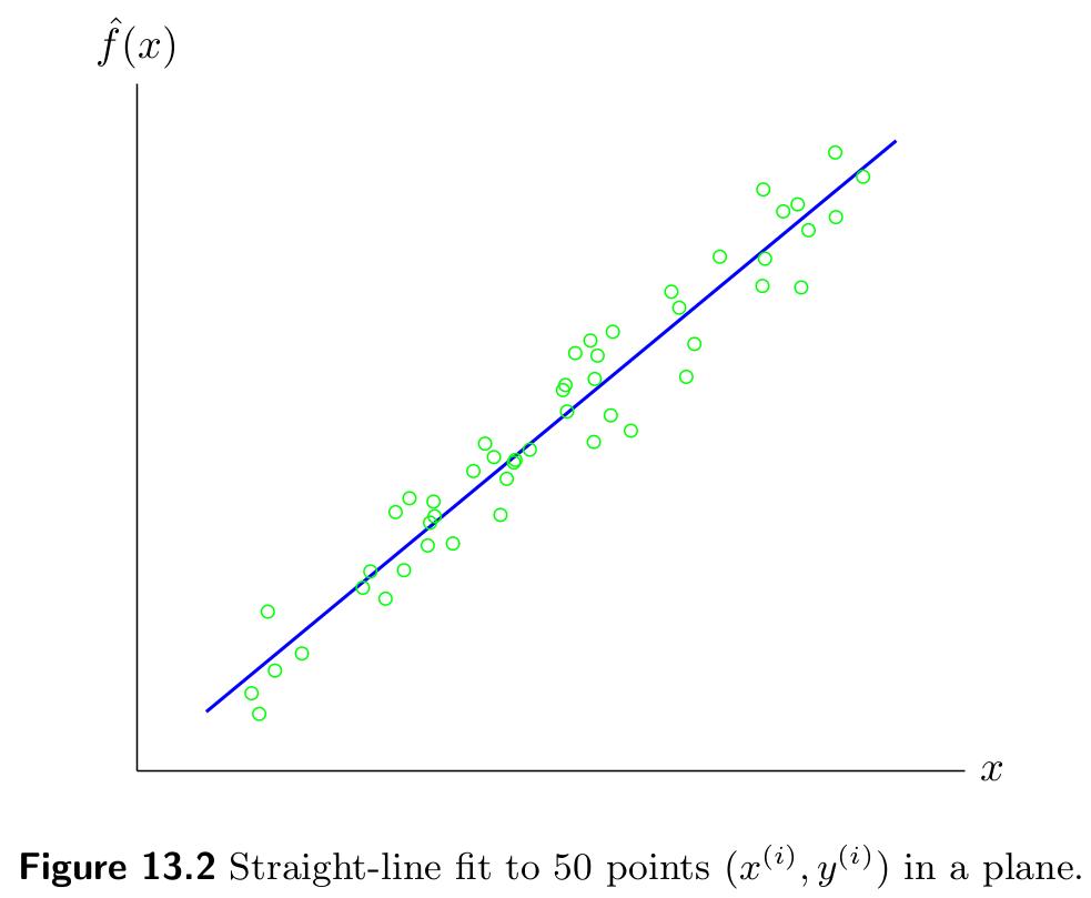
A = \begin{bmatrix} 1 & x^{(1)} \\ 1 & x^{(2)} \\ \vdots & \vdots \\ 1 & x^{(N)} \end{bmatrix}

(15)

Although we can work out formulas for $\hat{\theta}_1$ and $\hat{\theta}_2$ , they are not particularly interesting or informative. Instead, we’ll focus on some examples of how to use these ideas. A straight-line fit to 50 data points is given below.

7Univariate Function: Polynomial Fit¶

A simple extension beyond the straight-line fit is a polynomial fit where we set the $j^{th}$ feature to be

f_j(x) = x^{j-1}

(16)

for $j = 1,\ldots,p$ . This leads to a model class composed of polynomials of at most degree $p-1$ :

\hat{f}(x) = \theta_1 + \theta_2 x + \theta_3 x^2 + \cdots + \theta_p x^{p-1}

(17)

In this case, our matrix $A \in \mathbb{R}^{N \times p}$ and takes the form

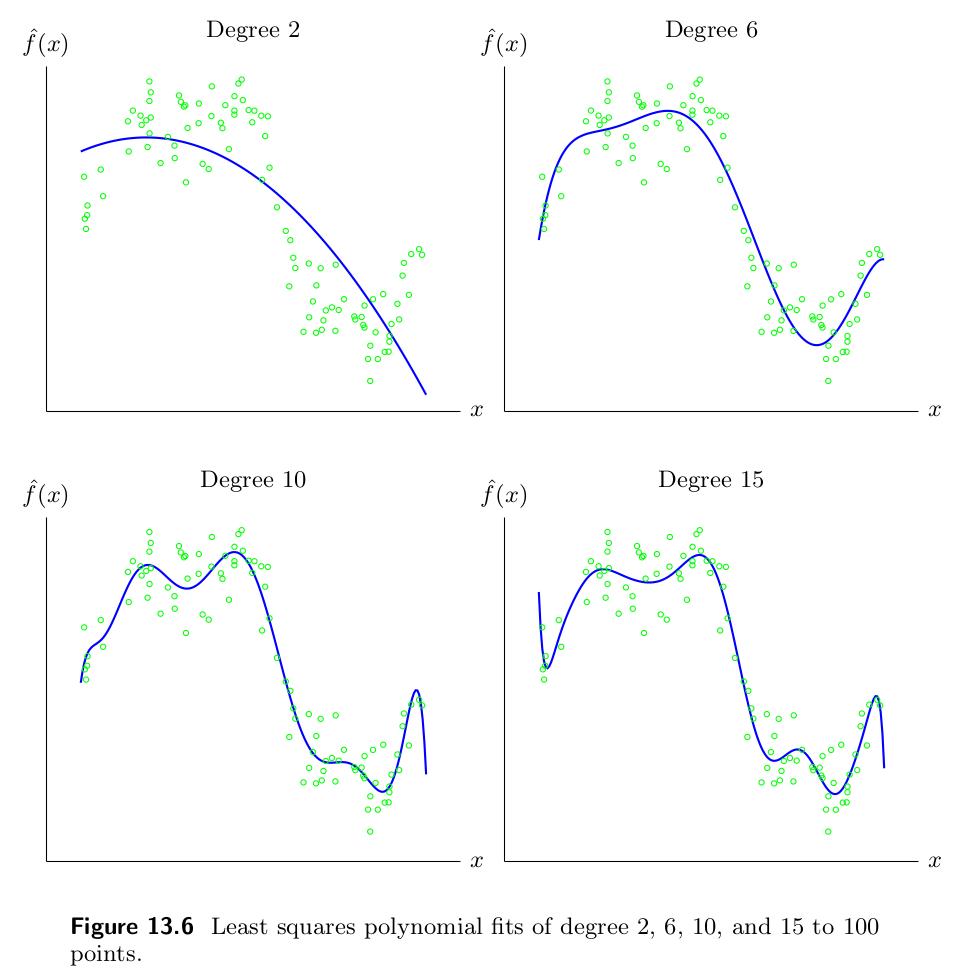
A = \begin{bmatrix} 1 & x^{(1)} & \cdots & (x^{(1)})^{p-1} \\ 1 & x^{(2)} & \cdots & (x^{(2)})^{p-1} \\ \vdots & \vdots & \ddots & \vdots \\ 1 & x^{(N)} & \cdots & (x^{(N)})^{p-1} \end{bmatrix}

(18)

which you might recognize as a Vandermonde Matrix, which we encountered earlier in the class when discussing polynomial interpolation. An important property of such matrices is that their columns are linearly independent provided that the numbers $x^{(1)}, \ldots, x^{(N)}$ include at least $p$ different values. The figures below show examples of least squares fits of polynomials of degree 2, 6, 10, and 15 to a set of 100 data points.

8Regression Models¶

We now consider the setting of vector-valued independent variables ${\vv x \in \mathbb{R}^n}$ . The analog of a straight-line fit here is a linear regression model of the form:

\hat{y} = \hat{f}(\vv x) = \boldsymbol \beta^{\top} \vv x + v,

(19)

where $\boldsymbol\beta \in \mathbb{R}^{n}$ and $v \in \mathbb{R}$ . If we set $\theta = \begin{bmatrix} v \\ \boldsymbol \beta \end{bmatrix}$ , then the model becomes:

\hat{y} = \theta_1 + \theta_2 x_1 + \cdots + \theta_{n+1} x_n.

(20)

We can view this as fitting within our general linear in the parameters model by setting $f_1(\vv x) = 1$ and $f_i(\vv x) = x_{i-1}$ for $i = 2, \ldots, n+1$ , so that $p = n+1$ .

We are of course not obliged to use these features. Instead, suppose that we have $p-1$ features $f_2(\vv x), \ldots, f_p(\vv x)$ , and assume we have set $f_1(x) = 1$ , as is common done. If we define:

\tilde{\vv x} = \begin{bmatrix} f_2(x) \\ \vdots \\ f_p(x) \end{bmatrix} \in \mathbb{R}^{p-1}

(21)

we can write a linear regression model in the new feature vector $\tilde{\vv x}$ :

\hat{y} = \theta_1 f_1(\vv x) + \cdots + \theta_p f_p(\vv x) = \boldsymbol \beta^{\top} \tilde{\vv x} + v

(22)

where:

$\tilde{\vv x} = (f_2(\vv x), \ldots, f_p(\vv x))$ are the transformed features
$v = \theta_1$ is called the affine term
$\boldsymbol\beta = (\theta_2, \theta_3, \ldots, \theta_p)$ is the linear term

8.1Application: Auto-Regressive Time Series Modeling¶

Here is a very widely used application of the above ideas in the context of time-series forecasting. Our goal here is to fit a model that predicts elements of a time series $z_1, z_2, \ldots,$ where $z_t \in \mathbb{R}$ is a scalar quantity of interest.

A standard approach is to use an auto-regressive (AR) prediction model:

\hat{z}_{t+1} = \theta_1 z_t + \theta_2 z_{t-1} + \cdots + \theta_M z_{t-M+1}, \quad t = M, M+1, \ldots \quad (AR)

(23)

In equation (AR), the parameter $M$ is the memory of the model, and $\hat{z}_{t+1}$ is the prediction of the next value based on the previous $M$ observations. We will choose $\boldsymbol \theta \in \mathbb{R}^M$ to minimize

(\hat{z}_{M+1} - z_{M+1})^2 + \cdots + (\hat{z}_{T} - z_{T})^2

(24)

We can fit this within our regression model framework by

y^{(i)} = z_{M+i}, \quad \vv x^{(i)} = \begin{bmatrix} z_{M+i-1} \\ z_{M+i-2} \\ \vdots \\ z_{i} \end{bmatrix} \in \mathbb{R}^M, \quad i = 1, \ldots, T-M.

(25)

A little bit of bookkeeping allows us to conclude that we have ${N = T-M}$ examples and $p = M$ features.

Example 2 (LAX Temperature Prediction)

As an example, consider the time series of hourly temperature at Los Angeles International Airport, May 1-31, 2016, with length $31 \cdot 24 = 744$ . The simple constant prediction $\hat{z}_{t+1} = 61.76^o \ \text{F}$ (the average temperature) has RMS prediction error $3.05^o \ \text{F}$ (the standard deviation). The very simple predictor $\hat{z}_{t+1} = z_t$ , i.e., guessing that the temperature next hour is the same as the current temperature, has RMS error $1.16^o \ \text{F}$ . The predictor $\hat{z}_{t+1} = z_{t-23}$ , i.e., guessing that the temperature next hour is what is was yesterday at the same time, has RMS error $1.73^o \ \text{F}$ .

We fit an AR model with memory $M=8$ using least squares, with $N=31 \cdot 24 - 8 = 736$ samples. The RMS error of this predictor is $0.98^o \ \text{F}$ , smaller than the RMS errors for the simple predictors described above. This figure shows the temperature and the predictions for the first five days.

Python break!¶

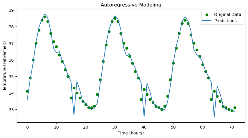
In the following code, we show how to fit an auto-regressive model to an online temperature data set that is given in an excel sheet (.csv file). Typically, such large data sets are stored as pandas DataFrame in Python. We convert the pandas DataFrame to numpy format and create our data for the auto-regressive model for a given memory. Then, we use np.linalg.lstsq to solve the least squares problem as we did before.

import pandas as pd
import numpy as np
import matplotlib.pyplot as plt

# Data source: https://www.ncei.noaa.gov/cdo-web/search
# Read CSV file into pandas DataFrame
df = pd.read_csv('LGA_temp.csv') # Temperature at LGA airport for 2010 (12 months)
temp = df['HLY-TEMP-NORMAL'].to_numpy()

memory = 8
T = temp.size
N = T - memory

# Function to create the dataset for AR model
def create_data(data, M):
    X, y = [], []
    for i in range(M, len(data)):
        X.append(data[i-M:i])
        y.append(data[i])
    return np.array(X), np.array(y)

# Create lagged dataset
X_data, y_data = create_data(temp, memory)

theta, residual, rank, sing_val = np.linalg.lstsq(X_data, y_data, rcond=None)
y_pred = X_data @ theta

print("RMS error: ", np.sqrt(residual/N))
# Plot predictions
plot_hours = 24*3 # first 3 days of 2010
plt.figure(figsize=(10, 5))
plt.scatter(np.arange(plot_hours), y_data[:plot_hours], color='green', label='Original Data')
plt.plot(y_pred[:plot_hours], label='Predictions')
plt.xlabel('Time (hours)')
plt.ylabel('Temprature (Fahrenheit)')
plt.title('Autoregressive Modeling')
plt.legend()
plt.show()

RMS error:  [0.34101808]

9Model Selection, Generalization, and Validation¶

This section is entirely practical: these are standard “tricks of the trade” that you will revisit in more detail in mae advanced classes on statistics and machine learning.

Our starting point is a philosophical question: what is the foul of a learned model? Perhaps surprisingly, it is NOT TO PREDICT OUTCOMES FOR THE GIVEN DATA; after all, we already have this data! Instead, we want to predict the outcome on new, unseen data.

If a model makes reasonable predictions on new unseen data, it is said to generalize. On the other hand, a model that makes poor predictions on new unseen data, but predicts the given data well, is said to be over-fit.

Then, we only use the training data to fit (or “train”) our model, and then evaluate the model’s performance on the test set. If the prediction errors on the training and test sets are similar, then we guess the model will generalize. This is rarely guaranteed, but such a comparison is often predictive of a model’s generalization properties.

Validation is often used for model selection, ie., to choose among different candidate models. For example, by comparing train/test errors, we can select between;

Polynomial models of different degrees.
Regression models with different sets of features
AR models with different memories.

Python break!¶

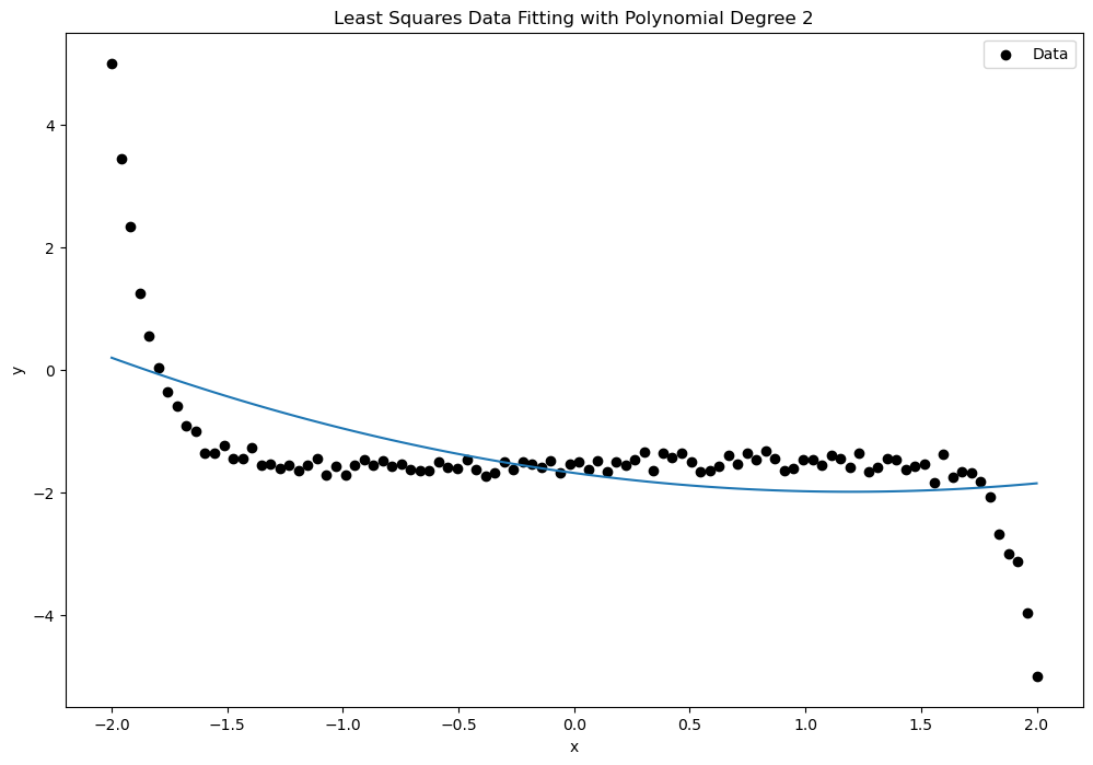
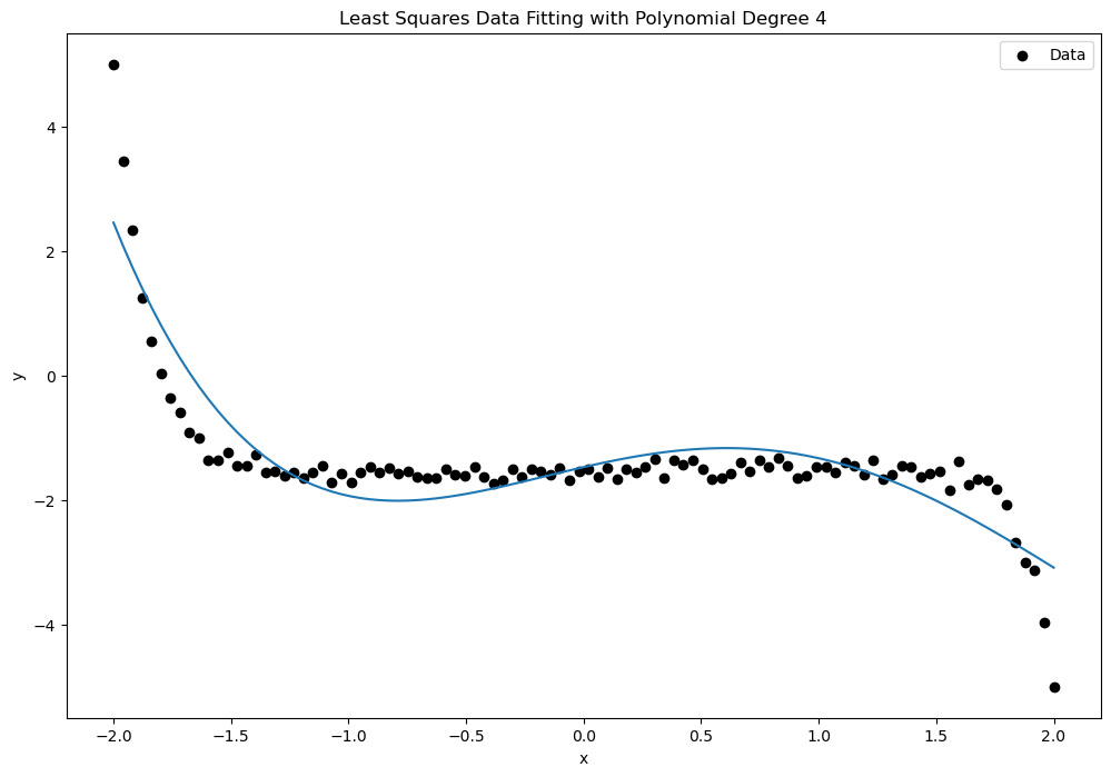
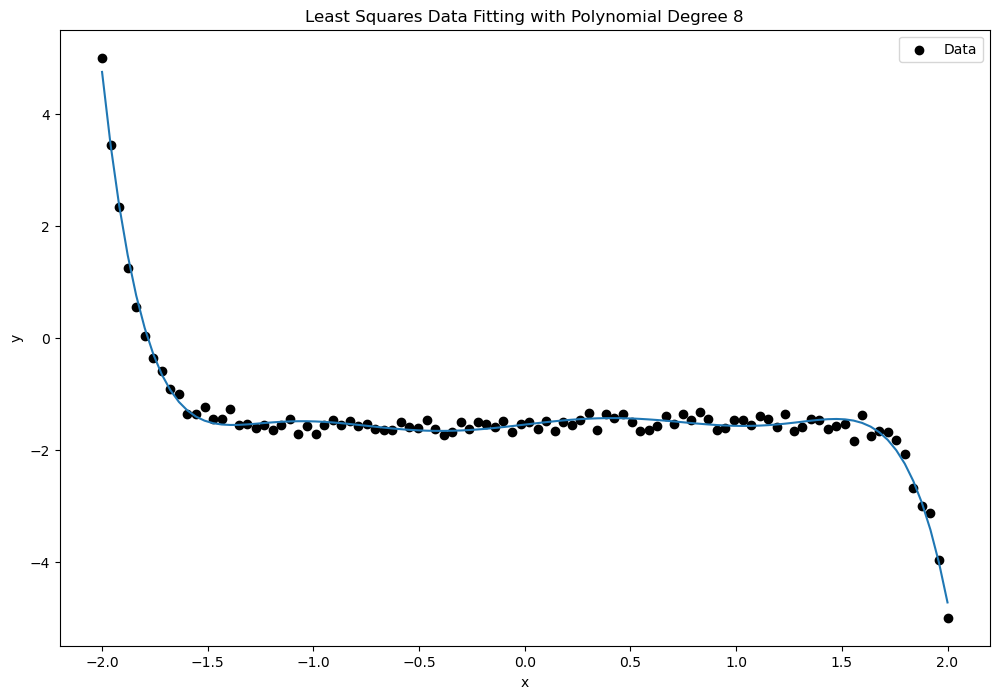
In the following code, we use the polyfit function from the Polynomial libray in Python to fit a polynomial model by solving the corresponding least squares problem. We compare the RMS error and the quality of fit for varying degrees of polynomial using synthetic data.

import numpy as np
import matplotlib.pyplot as plt
from numpy.polynomial.polynomial import Polynomial

# Generate synthetic data
np.random.seed(334)
x = np.linspace(-2, 2, 100)
y = -0.5*x**13 + x**10 + 2*x**9 - x**7  + 0.3*x**6 - 3*x**4 + 2 * x**3 - 5 * x**2 + 3 * x + np.random.normal(0, 10, size=x.shape)*7
y_data = ((y - min(y))/(max(y) - min(y)))*10 - 5 # scaling to [-5, 5]
# Function to fit and plot polynomials of varying degrees
def fit_and_plot_polynomial(x, y, degrees):

    
    for degree in degrees:
        # Fit polynomial of given degree
        p, results = Polynomial.fit(x, y, degree, full=True) # results[0] is residuals
        y_fit = p(x)

        print(f'RMS for Degree {degree}: ', np.sqrt(results[0]/y.size))
        plt.figure(figsize=(12, 8))
        plt.scatter(x, y, label='Data', color='black')
        # Plot the polynomial fit
        plt.plot(x, y_fit)
    
        plt.xlabel('x')
        plt.ylabel('y')
        plt.title(f'Least Squares Data Fitting with Polynomial Degree {degree}')
        plt.legend()
        plt.show()

# Degrees of polynomials to fit
degrees = [2, 4, 8, 10]

# Fit and plot polynomials
fit_and_plot_polynomial(x, y_data, degrees)

RMS for Degree 2:  [0.89961455]

RMS for Degree 4:  [0.53118696]

RMS for Degree 8:  [0.12656145]

RMS for Degree 10:  [0.10145153]