9.4 Graph Theory - Consensus

1Reading¶

Material related to this page can be found in

2Learning Objectives¶

By the end of this page, you should know:

what is a consensus protocol
the consensus theorem
how the eigenvalues/eigenvectors of the Laplacian matrix relate to consensus in a graph

3Consensus Protocols¶

Consider a collection of $N$ agents that communicate along a set of undirected links described by a graph $G$ . Each agent has state $x_i(t) \in \mathbb{R}$ , with initial value $x_i(0)$ , and together, they wish to determine the average of the initial states $\text{avg}(\vv x(0)) = \frac{1}{N} \sum_{i=1}^N x_i(0)$ .

The agents implement the following consensus protocol:

\dot{x}_i = \sum_{j \in N_i} (x_j - x_i) = -|N_i| (x_i - \text{avg}(x_{N_i})),

(1)

where $\text{avg}(x_{N_i}) = \frac{1}{|N_i|} \sum_{j \in N_i} x_j$ is the average of the states of the neighbors of agent $i$ . This is equivalent to the first-order homogeneous linear ordinary differential equation:

\dot{\vv x} = -L\vv x. \quad (\text{AVG})

(2)

Based on our previous analysis of such systems, we know that the solution to (AVG) is given by

\vv x(t) = c_1 e^{\lambda_1 t} \vv v_1 + \cdots + c_n e^{\lambda_n t} \vv v_n, \quad \vv x(0) = \bm \vv v_1 & \cdots & \vv v_n \em \vv c. \quad (\text{SOL})

(3)

where $(\lambda_i, \vv v_i)$ , $i=1,\ldots,n$ , are the eigenvalue/eigenvector pairs of the negative graph Laplacian $-L$ . Thus, the behavior of the consensus system (AVG) is determined by the spectrum of $L$ . We will spend the rest of this lecture on understanding the following theorem:

This result is extremely intuitive! It says that so long as the information at one node can eventually reach every other node in the graph, then we can achieve consensus via the protocol (AVG). Let’s try to understand why. As in the previous lecture, we order the eigenvalues of $-L$ in decreasing order: $\lambda_1 \geq \lambda_2 \geq \cdots \geq \lambda_n$ .

Our first observation is that $\lambda_1 = 0$ , $\vv v = \vv 1$ is an eigenvalue/eigenvector pair for $-L$ . This follows from the fact that each row of $L$ sums to 0, and so:

-L \mathbf{1} = \mathbf{0} = 0 \mathbf{1}.

(4)

A fact that we’ll show is true later is that the eigenvalues of $L$ are all nonnegative, and thus we know that $\lambda_i \leq 0$ for the eigenvalues of $-L$ . As such, we know that $\lambda = 0$ is the largest eigenvalue of $-L$ : hence we label them $\lambda_1 = 0$ , $\vv v_1 = \mathbf{1}$ .

Next, we recall that for an undirected graph, the Laplacian $L$ is symmetric, and hence is diagonalized by an orthonormal eigenbasis $-L = Q \Lambda Q^T$ , where $Q = \bm \vv u_1 & \cdots & \vv u_n\em$ is an orthogonal matrix composed of orthonormal eigenvectors of $L$ , and $\Lambda = \text{diag}(\lambda_1, \ldots, \lambda_n)$ . Although we do not know $\vv u_2, \ldots, \vv u_n$ , we know that $\vv u_1 = \frac{\vv v_1}{\|\vv v_1\|}\frac{1}{\sqrt{N}} \mathbf{1}$ .

We can therefore rewrite (SOL) as:

\begin{align*} \vv x(t) &= c_1 e^{0t} \frac{1}{\sqrt{N}} \mathbf{1} + c_2 e^{\lambda_2 t} \vv u_2 + \cdots + c_n e^{\lambda_n t} \vv u_n \\ &= c_1 \frac{1}{\sqrt{N}} \mathbf{1} + c_2 e^{\lambda_2 t} \vv u_2 + \cdots + c_n e^{\lambda_n t} \vv u_n \end{align*}

(5)

where now we can compute $\vv c$ by solving $\vv x(0) = Q\vv c \Rightarrow \vv c = Q^T \vv x(0)$ , as $Q$ is an orthogonal matrix.

Let’s focus on computing $c_1$ :

c_1 = \vv u_1^T \vv x(0) = \frac{1}{\sqrt{N}} \mathbf{1}^T \vv x(0) = \frac{1}{\sqrt{N}} \sum_{i=1}^N x_i(0).

(6)

Plugging this back into (5), we get:

\begin{align*} \vv x(t) &= \frac{1}{N} \sum_{i=1}^N x_i(0) \cot \mathbf{1} + c_2 e^{\lambda_2 t} \vv u_2 + \cdots + c_n e^{\lambda_n t} \vv u_n \\ &= \text{avg}(\vv x(0)) \mathbf{1} + c_2 e^{\lambda_2 t} \vv u_2 + \cdots + c_n e^{\lambda_n t} \vv u_n. \end{align*}

(7)

This is very exciting! We have shown that the solution $\vv x(t)$ to (AVG) is composed of a sum of the final consensus state $\vv x^* = \text{avg}(\vv x(0)) \mathbf{1}$ and exponential functions $c_i e^{\lambda_i t} \vv u_i$ , $i=2,\ldots,n$ , evolving in the subspace $\vv u_1^\perp$ orthogonal to the consensus direction $\frac{1}{\sqrt{N}} \mathbf{1}$ . Thus, if we can show that $\lambda_2, \ldots, \lambda_n < 0$ , we will have established our result.

To establish this result, we start by stating a widely used theorem for bounding localizing eigenvalues.

Theorem 2 (Gershgorin’s Disk Theorem)

Let $A \in \mathbb{R}^{n \times n}$ and define the radius

r_i = \sum_{j=1, j \neq i}^n |a_{ij}|

(8)

as the absolute row sum with entry $a_{ii}$ deleted. Then all eigenvalues of $A$ are located in the union of $n$ disks:

G(A) = \bigcup_{i=1}^n G_i(A), \quad G_i(A) = \{z \in \mathbb{C} \mid |z - a_{ii}| \leq r_i\}

(9)

In the case of symmetric matrices, we can restrict the $G_i(A)$ to the real line:

G_i(A) = \{\lambda \in \mathbb{R} \mid |\lambda - a_{ii}| \leq r_i\}

(10)

Let’s apply this theorem to a graph Laplacian $L$ . The diagonal elements of $L = \Delta - A$ are given by $\Delta_{ii} = \text{out}(v_i)$ , the out-degree of node $i$ . Further, the radii $r_i = \text{out}(v_i)$ as well, as $a_{ij} = 1$ if node $i$ is connected to node $j$ , and 0 otherwise. Therefore, for row $i$ , we have the following Gershgorin intervals:

G_i(L) = \{\lambda \in \mathbb{R} \mid |\lambda - \text{out}(v_i)| \leq \text{out}(v_i)\}.

(12)

These are intervals of the form $[0, 2\text{out}(v_i)]$ , and therefore the union $G(L) = \bigcup_{i=1}^n G_i(L) = [0, 2d_{\text{max}}]$ , where $d_{\text{max}} = \max_i \text{out}(v_i)$ is the maximal out degree of a node in the graph. Taking the negative of everything, we conclude that $G(-L) = [-2d_{\text{max}}, 0]$ .

This tells us that $\lambda_i \leq 0$ for $i=1,2,\ldots,n$ for the eigenvalues of $-L$ . This is almost what we wanted. We still need to show that only $\lambda_1 = 0$ and that $\lambda_n \leq \cdots \leq \lambda_2 < 0$ . To answer this question, we rely on the following proposition:

Unfortunately proving this result would take us too far astray. Instead, we highlight the intuitive nature of the result in terms of the consensus system (AVG). This proposition tells us that if the communication graph $G$ is strongly connected, i.e., if everyone’s information eventually reaches everyone, then $\vv x(t) \to \vv x^* = \text{avg}(\vv x(0))\mathbf{1}$ at a rate governed by the slowest decaying node $e^{-\lambda_2 t}$ .

In contrast, suppose the graph $G$ is disconnected, and consists of the disjoint union of two connected graphs $G_1 = (\mathcal{V}_1, \mathcal{E}_1)$ and $G_2 = (\mathcal{V}_2, \mathcal{E}_2)$ , i.e., $G = (\mathcal{V}_1 \cup \mathcal{V}_2, \mathcal{E}_1 \cup \mathcal{E}_2)$ and $\mathcal{V}_1 \cap \mathcal{V}_2 = \emptyset$ and $\mathcal{E}_1 \cap \mathcal{E}_2 = \emptyset$ . Then if we run the consensus protocol (AVG) on $G$ , the system effectively decouples into two parallel systems, each evolving on their own graph and blissfully unaware of the other:

\dot{\vv x}_1 = -L_1 \vv x_1 \quad \text{and} \quad \dot{\vv x}_2 = -L_2 \vv x_2.

(13)

Here we use $\vv x_1$ to denote the state of agents in $G_1$ , with Laplacian $L_1$ , and similarly for $\vv x_2$ . By the above discussion, if $L_1$ and $L_2$ are both strongly connected, then $\vv x_i(t) \to \text{avg}(\vv x_i(0)) \mathbf{1}$ , and $\lambda = 0, \vv v = \mathbf{1}$ is an eigenvalue/vector pair for each graph.

If we now consider the joint graph $G$ composed of the two disjoint graphs $G_1$ and $G_2$ , we can immediately see how to change our consensus protocol: $\dot{\vv x}_i = -L_i\vv x_i$ will evolve as it did before.

To see how this manifests in the algebraic multiplicity of the 0 eigenvalue of $L = \begin{bmatrix} L_1 & \\ & L_2 \end{bmatrix}$ , note that for the composite system with state $\vv x = \begin{bmatrix} \vv x_1 \\ \vv x_2 \end{bmatrix}$ , we have the consensus dynamics:

\begin{bmatrix} \dot{\vv x}_1 \\ \dot{\vv x}_2 \end{bmatrix} = \begin{bmatrix} -L_1 & \\ & -L_2 \end{bmatrix} \begin{bmatrix} \vv x_1 \\ \vv x_2 \end{bmatrix},

(14)

which has $\lambda_1 = 0$ with $\vv v_1 = \begin{bmatrix} \vv 1 \\ \vv 0 \end{bmatrix}$ and $\lambda_2 = 0$ with $v_2 = \begin{bmatrix} \vv 0 \\ \vv 1 \end{bmatrix}$ so that:

\begin{bmatrix} \vv x_1^* \\ \vv x_2^* \end{bmatrix} = \begin{bmatrix} \vv 1 \\ \vv 0 \end{bmatrix} \text{avg}(\vv x_1(0)) + \begin{bmatrix} \vv 0 \\ \vv 1 \end{bmatrix} \text{avg}(\vv x_2(0)).

(15)

This is of course expected, as all we have done is rewrite (13) using block vectors and matrices --- we have not changed anything about the consensus protocol.

4Python Break: Determining if a Graph is Connected!¶

In this section, let’s look at an efficient algorithm to check if an (undirected) graph $G$ is connected, i.e., has exactly one connected component. Of course, we showed above that the zero eigenvalue has algebraic multiplicity one in the Laplacian of $G$ if and only if $G$ is connected, which gives us one avenue of attack: to find the eigenvalues of $G$ .

In this section, we will explore how a much simpler class of algorithms, known as graph traversal algorithms, can be used to find the connected components of a graph (and count how many there are). The particular class of algorithm we will look at are called tree-based graph traversal algorithms. At a high level, the algorithm starts maintains a set of visited vertices, and at each step, chooses an unvisited vertex that is adjacent to a visited vertex and visits it; the algorithm starts at an arbitrary vertex. A visual can be found below:

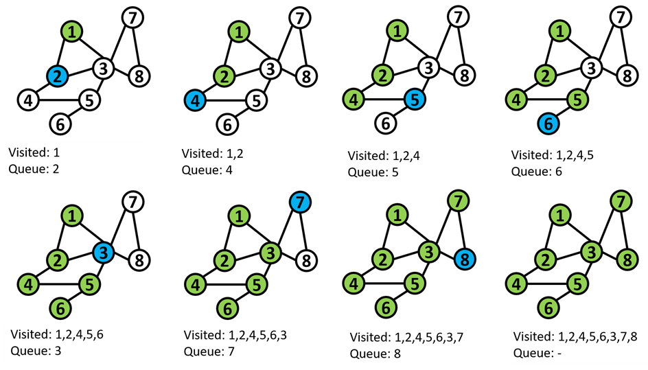
From left to right, top to bottom, we see that at each iteration, we choose a vertex (marked in blue) that is adjacent to a green vertex and make it green (visit it). If we start this procedure from a vector $v$ , then this procedure will in fact visit all vertices in the connected component of $v$ . Try to convince yourself of this fact! To start, recall that $u$ is in the connected component of $v$ if and only if there is a path $P = v\to \dots \to u$ from $v$ to $u$ in the graph.

Below, we have an implementation of this procedure in Python:

import random
from random import randrange
random.seed(6928)

class Graph:
    def __init__(self, n):
        self.n_vertices = n
        self.neighbors = [set() for _ in range(n)]

    def add_edge(self, i, j):
        self.neighbors[i].add(j)
        self.neighbors[j].add(i)

    def n_edges(self):
        return int(sum([len(s) for s in self.neighbors]) / 2)
    
    def print_edges(self):
        for v in range(self.n_vertices):
            for neighbor in self.neighbors[v]:
                if neighbor > v:
                    print('(' + str(v) + ', ' + str(neighbor) + ')')

    def connected_component(self, v):
        cc = set()

        visited = [False for _ in range(self.n_vertices)]
        frontier = [v]

        while len(frontier) > 0:
            index = randrange(len(frontier))
            v = frontier.pop(index)
            if visited[v]:
                continue

            visited[v] = True
            cc.add(v)
            for neighbor in self.neighbors[v]:
                frontier.append(neighbor)

        return cc

g = Graph(5)
g.add_edge(0, 1)
g.add_edge(1, 2)
g.add_edge(2, 0)
g.add_edge(3, 4)

print('Edges of g:')
g.print_edges()
print('Connected component of 0:', g.connected_component(0))
print('Connected component of 1:', g.connected_component(1))
print('Connected component of 2:', g.connected_component(2))
print('Connected component of 3:', g.connected_component(3))
print('Connected component of 4:', g.connected_component(4))

print()

h = Graph(5)
h.add_edge(0, 1)
h.add_edge(1, 2)
h.add_edge(2, 0)
h.add_edge(3, 4)
h.add_edge(0, 4)

print('Edges of h:')
h.print_edges()
print('Connected component of 0:', h.connected_component(0))
print('Connected component of 1:', h.connected_component(1))
print('Connected component of 2:', h.connected_component(2))
print('Connected component of 3:', h.connected_component(3))
print('Connected component of 4:', h.connected_component(4))

Edges of g:
(0, 1)
(0, 2)
(1, 2)
(3, 4)
Connected component of 0: {0, 1, 2}
Connected component of 1: {0, 1, 2}
Connected component of 2: {0, 1, 2}
Connected component of 3: {3, 4}
Connected component of 4: {3, 4}

Edges of h:
(0, 1)
(0, 2)
(0, 4)
(1, 2)
(3, 4)
Connected component of 0: {0, 1, 2, 3, 4}
Connected component of 1: {0, 1, 2, 3, 4}
Connected component of 2: {0, 1, 2, 3, 4}
Connected component of 3: {0, 1, 2, 3, 4}
Connected component of 4: {0, 1, 2, 3, 4}

Above, we define two graphs g and h and find the connected component corresponding to each vertex in the two graphs using the connected_components function. Note that g has two connected components, {0, 1, 2} and {3, 4} whereas h has only one connected component {0, 1, 2, 3, 4}, meaning that h is connected and g is not.

Let’s understand how this algorithm implements the procedure we described above. At a high level, at each iteration of the while loop, the cc set will contain all the vertices we have already visited (the visited array will also indicate which vertices we have already visited), and the frontier list will contain all the unvisited vertices adjacent to any vertex we have already visited. At each iteration of the while loop, we pick a random vertex in the frontier list and visit it, and then repeat until there are no more vertices to explore (i.e., we have explored the entire connected component). At the end of this procedure, the cc set will contain all the vertices in our connected component!

To conclude, we have a few remarks about the way we choose vertices from the frontier list. Currently, we randomly select vertices from this list, but we can instead use an arbitrary rule to choose which vertex instead. For example:

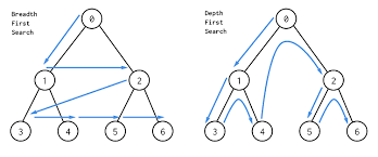
If we choose the vertex in frontier which was added earliest (out of all vertices which are in frontier), then this algorithm is called breadth-first search, or BFS.
If we choose the vertex in frontier which was most recently added, then this algorithm is called depth-first search, or DFS.

A visual of BFS versus DFS is below:

If you take a computer science class, you’ll definitely see these very commonly used algorithms in a lot more detail!