7.1 Complex Eigenvalues and Linear Dynamical Systems

0.1Reading¶

Material related to this page, as well as additional exercises, can be found in ALA 10.1 and 10.3.

0.2Learning Objectives¶

By the end of this page, you should know:

how to use Euler’s formula,
how to write real solutions to linear dynamical systems that have complex eigenvalues.

1Solving Linear ODEs with Complex Eigenvalues¶

In the previous section on linear ODEs, we learned how to find the solutions when the coefficient matrix $A$ was diagonalizable. We also saw some examples when $A$ was diagonalizable and had all real eigenvalues. It turns out that the same procedure generalizes when $A$ is diagonalizable, but has complex eigenvalues. On this page, we’ll see how this can be done.

Let’s apply our solution method for diagonalizable $A$ to $\dot{\vv x} = A \vv x$ with $A = \begin{bmatrix} 0 & -1 \\ 1 & 0 \end{bmatrix}$ . We are given that $A$ has eigenvalue/eigenvector pairs:

\lambda_1 = i, \ \vv v_1 = \begin{bmatrix} 1 \\ -i \end{bmatrix} \quad \text{and} \quad \lambda_2 = -i, \vv v_2 = \begin{bmatrix} 1 \\ i \end{bmatrix}.

(1)

Even though these eigenvalues/vectors have complex entries, we can still use our solution method for diagonalizable $A$ ! We write the solution to $\dot{\vv x} = A\vv x$ as

\vv x(t) = c_1e^{\lambda_1 t}\vv v_1 + c_2e^{\lambda_2t}\vv v_2 = c_1e^{it}\begin{bmatrix} 1 \\ -i \end{bmatrix} + c_2e^{-it}\begin{bmatrix} 1 \\ i \end{bmatrix}, \quad (\text{SOL})

(2)

i.e., $\vv x(t)$ is a linear combination of the two solutions

\vv x_1(t) = c_1e^{it}\begin{bmatrix} 1 \\ -i \end{bmatrix} \quad \text{and} \quad \vv x_2(t) = c_2e^{-it}\begin{bmatrix} 1 \\ i \end{bmatrix}. \quad (\text{BASE})

(3)

and then solve for $c_1$ and $c_2$ to ensure compatibility with the initial condition $\vv x(0)$ . In general $c_1$ and $c_2$ will also be complex numbers, and $\vv x(t)$ will take complex values. This is mathematically correct, and indeed one can study dynamical systems evolving over complex numbers. However, we will see that with a little massaging, we can rewrite this solution in a more useful form!

1.1Rewriting the Solution to a Linear ODE¶

In this class, and in most engineering applications, we are interested in real solutions to $\dot{\vv x} = A\vv x$ . If we know want real solutions, it might make sense to try to find different “base” solutions than $\vv x_1(t)$ and $\vv x_2(t)$ that still span all possible solutions to $\dot{\vv x} = A\vv x$ . Our key tool for accomplishing this is Euler’s formula:

We apply Euler’s formula to (BASE), and obtain (after simplifying):

\begin{align*} \vv x_1(t) = e^{it}\begin{bmatrix} 1 \\ -i \end{bmatrix} = \begin{bmatrix} \cos t \\ \sin t \end{bmatrix} + i\begin{bmatrix} \sin t \\ -\cos t \end{bmatrix}, \vv x_2(t) = e^{-it}\begin{bmatrix} 1 \\ i \end{bmatrix} = \begin{bmatrix} \cos t \\ \sin t \end{bmatrix} - i\begin{bmatrix} \sin t \\ -\cos t \end{bmatrix}. \end{align*}

(4)

We’ve made some progress, in that $\vv x_1(t)$ and $\vv x_2(t)$ are now in the “standard” complex number form $a+ib$ , and that $\vv x_1(t) = \overline{\vv x_2}(t)$ , i.e., $\vv{x_1}(t)$ and $\vv{x_2}(t)$ are complex conjugates. We use this observation strategically to define two new “base” solutions:

\begin{align*} \hat{\vv x}_1(t) &= \frac{1}{2}(\vv x_1(t) + \vv x_2(t)) = \frac{1}{2}(\vv x_1(t) + \overline{\vv x_1}(t)) \\ &= \begin{bmatrix} \cos t \\ \sin t \end{bmatrix} (= \text{Re}\{\vv x_1(t)\}) \end{align*}

(5)

\begin{align*} \hat{\vv x}_2(t) &= \frac{1}{2i}(\vv x_1(t) - \vv x_2(t)) = \frac{1}{2i}(\vv x_1(t) - \overline{\vv x_1}(t)) \\ &= \begin{bmatrix} \sin t \\ -\cos t \end{bmatrix} (= \text{Im}\{\vv x_1(t)\}) \end{align*}

(6)

We note that since $\hat{\vv x}_1(t)$ and $\hat{\vv x}_2(t)$ are linear combinations of $\vv x_1(t)$ and $\vv x_2(t)$ , they are valid solutions to $\dot{\vv x} = A\vv x$ . Furthermore, since $\hat{\vv x}_1(t)$ and $\hat{\vv x}_2(t)$ are linearly independent (i.e., $c_1\hat{\vv x}_1(t) + c_2\hat{\vv x}_2(t) = 0$ for all $t$ if and only if $c_1 = c_2 = 0$ ), they form a basis for the solution set to $\dot{\vv x} = A \vv x$ . Therefore, we can rewrite (SOL) as

\vv x(t) = c_1\begin{bmatrix} \cos t \\ \sin t \end{bmatrix} + c_2\begin{bmatrix} \sin t \\ -\cos t \end{bmatrix}

(7)

and then solve for $c_1$ and $c_2$ using $\vv x(0)$ . If $\vv x(0) \in \mathbb{R}^2$ , i.e., if the initial condition $\vv x(0)$ is real, then $c_1$ and $c_2$ will be too. For example, suppose $\vv x(0) = \begin{bmatrix} a \\ b \end{bmatrix}$ , with $a,b \in \mathbb{R}$ . Then:

\vv x(0) = c_1\begin{bmatrix} 1 \\ 0 \end{bmatrix} + c_2\begin{bmatrix} 0 \\ -1 \end{bmatrix} = \begin{bmatrix} c_1 \\ -c_2 \end{bmatrix} = \begin{bmatrix} a \\ b \end{bmatrix} \Rightarrow c_1 = a, c_2 = -b,

(8)

and

\vv x(t) = \begin{bmatrix} a\cos t - b\sin t \\ a\sin t + b\cos t \end{bmatrix} = \begin{bmatrix} \cos t & -\sin t \\ \sin t & \cos t \end{bmatrix}\begin{bmatrix} a \\ b \end{bmatrix} = R(t) \vv x(0),

(9)

i.e., the solution $\vv x(t)$ corresponds to the initial condition $\vv x(0)$ being rotated in a counterclockwise direction at a frequency of 1 rad/s.

Note

The key steps in the above procedure were:

Apply Euler’s formula to rewrite the base solutions as
$\vv x_1(t) = \text{Re}\{\vv x_1(t)\} + i\text{Im}\{\vv x_1(t)\}, x_2(t) = \overline{\vv x_1}(t) = \text{Re}\{\vv x_1(t)\} - i\text{Im}\{\vv x_1(t)\}$
(10)
Define new basic solutions by setting:
$\hat{\vv x}_1(t) = \text{Re}\{\vv x_1(t)\} \ \text{and} \ \hat{\vv x}_2(t) = \text{Im}\{\vv x_2(t)\}$
(11)
It turns out that this approach is completely general, and can be applied whenever you encounter complex eigenvalue/vectors (which always appear as complex conjugate pairs).

Example 1

Consider the linear dynamical system $\dot{\vv x} = A \vv x$ , where

A = \begin{bmatrix} 1 & 2 & 0 \\ 0 & 1 & -2 \\ 2 & 2 & -1 \end{bmatrix} \quad \text{and} \quad \vv x(0) = \begin{bmatrix} 2 \\ -1 \\ -2 \end{bmatrix}.

(12)

Using the formula for the determinant of a 3x3 matrix (you don’t need to memorize this!), we can compute the following eigenvalue/vector pairs:

\begin{aligned} \lambda_1 &= -1, & \lambda_2 &= 1 + 2i, & \lambda_3 &= 1 - 2i \\ \vv v_1 &= \begin{bmatrix} -1 \\ 1 \\ 1 \end{bmatrix}, & \vv v_2 &= \begin{bmatrix} 1 \\ i \\ 1 \end{bmatrix}, & \vv v_3 &= \begin{bmatrix} 1 \\ -i \\ 1 \end{bmatrix} \end{aligned}

(13)

and obtain the corresponding eigensolutions:

\vv x_1(t) = e^{-t}\begin{bmatrix} -1 \\ 1 \\ 1 \end{bmatrix}, \quad \vv x_2(t) = e^{(1+2i)t}\begin{bmatrix} 1 \\ i \\ 1 \end{bmatrix}, \quad \vv x_3(t) = e^{(1-2i)t}\begin{bmatrix} 1 \\ -i \\ 1 \end{bmatrix}.

(14)

Let’s apply Euler’s formula to $\vv x_2(t)$ (remember that $e^{(1+2i)t} = e^t e^{i(2t)}$ ):

\begin{align*} \vv x_2(t) &= e^{(1+2i)t}\begin{bmatrix} 1 \\ i \\ 1 \end{bmatrix} = e^t(\cos 2t + i\sin 2t)\begin{bmatrix} 1 \\ i \\ 1 \end{bmatrix} &= \begin{bmatrix} e^t\cos 2t \\ -e^t\sin 2t \\ e^t\cos 2t \end{bmatrix} + i\begin{bmatrix} e^t\sin 2t \\ e^t\cos 2t \\ e^t\sin 2t \end{bmatrix}. \end{align*}

(15)

This means another set of real eigensolutions to $\dot{\vv x} = A\vv x$ is

\begin{align*} \vv x_1(t) = e^{-t}\begin{bmatrix} -1 \\ 1 \\ 1 \end{bmatrix}, \quad \hat{\vv x}_2(t) &= \text{Re}\{\vv x_2(t)\} &= e^t\begin{bmatrix} \cos 2t \\ -\sin 2t \\ \cos 2t \end{bmatrix}, \\ \hat{\vv x}_3(t) &= \text{Im}\{\vv x_2(t)\} &= e^t\begin{bmatrix} \sin 2t \\ \cos 2t \\ \sin 2t \end{bmatrix}, \end{align*}

(16)

and a general solution can be written as

\vv x(t) = c_1\vv x_1(t) + c_2\hat{\vv x}_2(t) + c_3\hat{\vv x}_3(t) = \begin{bmatrix} -c_1e^{-t} + c_2e^t\cos 2t + c_3e^t\sin 2t \\ c_1e^{-t} - c_2e^t\sin 2t + c_3e^t\cos 2t \\ c_1e^{-t} + c_2e^t\cos 2t + c_3e^t\sin 2t \end{bmatrix}

(17)

We compute our constants $c_1, c_2, c_3$ by solving

\mathbf{x}(0) = \begin{bmatrix} -c_1 + c_2 \\ c_1 + c_3 \\ c_1 + c_2 \end{bmatrix} = \begin{bmatrix} 2 \\ -1 \\ -2 \end{bmatrix} \Rightarrow c_1 = -2, \quad c_2 = 0, \quad c_3 = 1

(18)

thus obtaining the specific solution to our original initial value problem as:

\mathbf{x}(t) = \begin{bmatrix} x_1(t) \\ x_2(t) \\ x_3(t) \end{bmatrix} = \begin{bmatrix} 2e^{-t} + e^t\sin 2t \\ -2e^{-t} + e^t\cos 2t \\ -2e^{-t} + e^t\sin 2t \end{bmatrix}.

(19)

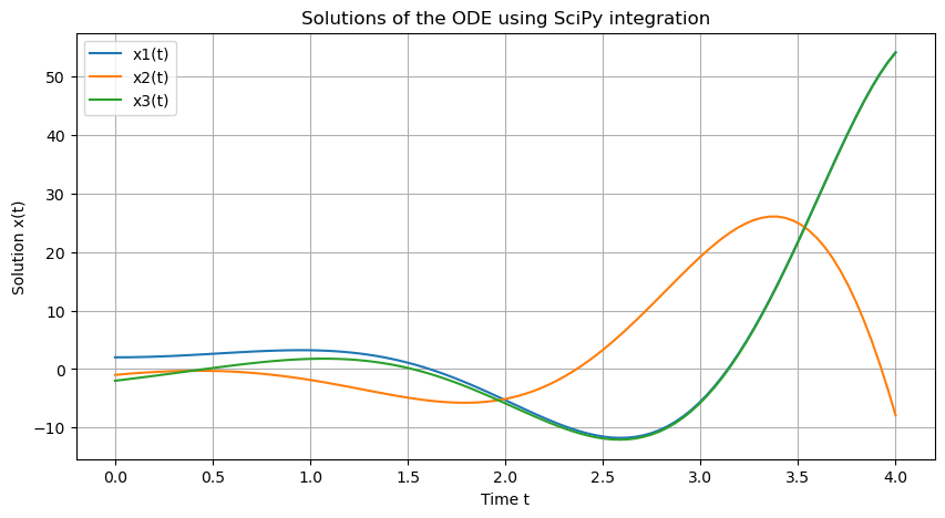
Python break!¶

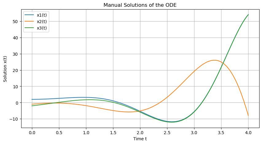
In the below code, we illustrate how to numerically integrate an ordinary differential equation using SciPy’s function in Python. We then compare it with the manual solution we obtained in Example 1.

import numpy as np
from scipy.integrate import solve_ivp
import matplotlib.pyplot as plt

A = np.array([[1, 2, 0],
          [0, 1, -2],
          [2, 2, -1]])

def system(t, x):
    return A @ x
    
x0 = np.array([2, -1, -2])

# Define time points for the solution
t_span = (0, 4)  # Time from 0 to 10
t_eval = np.linspace(t_span[0], t_span[1], 100)  # Time points where the solution is evaluated

# Solve the ODE system
sol = solve_ivp(system, t_span, x0, t_eval=t_eval)

# Extract the solution
times = sol.t
solutions = sol.y

# Plot the solutions
plt.figure(figsize=(10, 5))
plt.plot(times, solutions[0, :], label='x1(t)')
plt.plot(times, solutions[1, :], label='x2(t)')
plt.plot(times, solutions[2, :], label='x3(t)')
plt.xlabel('Time t')
plt.ylabel('Solution x(t)')
plt.title('Solutions of the ODE using SciPy integration')
plt.legend()
plt.grid()
plt.show()

## Manual solution from example 1

solutions_manual = np.vstack((2*np.exp(-times)+np.exp(times)*np.sin(2*times),
                             -2*np.exp(-times)+np.exp(times)*np.cos(2*times),
                              -2*np.exp(-times)+np.exp(times)*np.sin(2*times),))

# Plot the solutions
plt.figure(figsize=(10, 5))
plt.plot(times, solutions_manual[0, :], label='x1(t)')
plt.plot(times, solutions_manual[1, :], label='x2(t)')
plt.plot(times, solutions_manual[2, :], label='x3(t)')
plt.xlabel('Time t')
plt.ylabel('Solution x(t)')
plt.title('Manual Solutions of the ODE')
plt.legend()
plt.grid()
plt.show()