13.1 Unconstrained Optimization

1Reading¶

Material related to this page, as well as additional exercises, can be found in Chapter 12 in ROB101 textbook by Jesse Grizzle.

2Learning Objectives¶

By the end of this page, you should know

what is a mathematical optimization problem
the difference between constrained and unconstrained optimization
an example of optimization problem: least squares
what are local and global minimum
what are convex functions and some intuition on how to minimize them

3A Brief Introduction to Optimization¶

There were a few times during the semester where we tried to find the “best” vector (or matrix) among a collection of many such vectors or matrices. For example, in least squares, we looked to find the vector $\vv x$ that minimized the expression $\|A\vv x - b\|^2$ . In low-rank approximation, we looked to find the matrix $\hat{M}$ that has rank $k$ (or less) that minimized the expression $\|\hat{M} - M\|_F^2$ .

These were both specific instances of what is called a mathematical optimization problem. We will focus on unconstrained problems. You will learn a lot more about optimization problems in ESE 3040, and this lecture is only meant to give you a small taste, and to show how essential linear algebra is in finding solutions.

Optimization problem (1) is called unconstrained because we are free to pick any $\vv x \in \mathbb{R}^n$ we like to minimize $f(\vv x)$ . A constrained optimization problem has the additional requirement that $\vv x$ must satisfy some added conditions, e.g., live in the solution set of $A\vv x = b$ . We will not consider such problems in this lecture, but you’ll see many in ESE 3040.

The goal of optimization is to find a special decision variable $\vv x^*$ for which the cost function $f$ is as small as possible, i.e., such that

f(\vv x^*) \leq f(\vv x) \quad \text{for all } \vv x \in \mathbb{R}^n

(2)

Such an $\vv x^*$ is called an optimal solution to problem (1), and is defined as the arg min of $f$ :

\vv x^* = \arg\min_{\vv x \in \mathbb{R}^n} f(\vv x).

(3)

Equation (3) simply says in math that $\vv x^*$ satisfies the definition (2) of an optimal point.^[1]

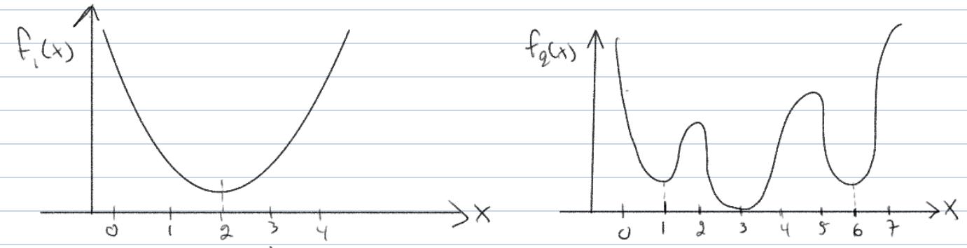
Despite how simple and innocuous problem (1) looks, it can be used to encode very rich and very challenging problems. Even for $\vv x \in \mathbb{R}$ , we can get ourselves into trouble. Consider the following two functions that we wish to minimize:

Which do you think is easier to optimize? The left figure, with function $f_1(x)$ , is “bowl-shaped” and is smallest at $x^* = 2$ . What’s “nice” about $f_1$ is that there’s also an obvious algorithm for finding $x^* = 2$ : If you imagine yourself as an ant standing on the function $f_1(x)$ , all you need to do is “walk downhill” until you eventually find the bottom of the bowl.

In contrast, the right figure with function $f_2(x)$ has many hills and valleys. The optimal value $x^* = 3$ is the one for which $f_2(x)$ is smallest. But now if we again imagine ourselves as an ant standing on the function $f_2(x)$ , our strategy of walking downhill will not always work! For example, if we were to start at $x = 1.5$ , then walking downhill would bring us to the bottom of the first valley at $x = 1$ . Now $x = 1$ is not an optimal point, since $f_2(3) < f_2(1)$ , but if we look around at nearby points, then $f_2(1)$ is indeed the smallest.

As you may have guessed, we really like “bowl-shaped” functions for which our walking downhill strategy finds a global minimum. Such functions satisfy a geometric property called convexity.

To understand what (CVX) is saying, it is best to draw what it means for a scalar function $f: \mathbb{R} \to \mathbb{R}$ .

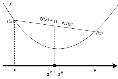
(CVX) says that if I pick any two points $f(x)$ and $f(y)$ on the graph, and draw a line segment between these two points, then this line lies above the graph. It turns out that this is exactly the right way to mathematically characterize “bowl-shaped” functions, even when $\vv x \in \mathbb{R}^n$ . The important feature of convex functions is that “walking downhill” will always bring us to a global minimum. We won’t say much more about convex functions, but you’ll see them again in ESE 3040, and there is a graduate level course, ESE 6050, which focuses entirely on convex optimization problems.

Example 2

The affine function $f(\vv x) = A\vv x - \vv b$ is convex. To see this, we check that

f(\theta \vv x + (1-\theta)\vv y) \leq \theta f(\vv x) + (1-\theta)f(\vv y) \text{ for all } \vv x, \vv y \in \mathbb{R}^n \text{ and } \theta \in [0,1]

But

f(\theta \vv x + (1-\theta)\vv y) = A(\theta \vv x + (1-\theta)\vv y) - \vv b = \theta (A\vv x - \vv b) + (1-\theta)(A\vv y - \vv b) = \theta f(\vv x) + (1-\theta)f(\vv y)

(7)

Affine functions are on the “boundary” of being convex, in the sense that if $f(\vv x)$ is an affine function, then $-f(\vv x)$ is also an affine function and hence is convex. Affine functions are the only functions $f$ for which both $f$ and $-f$ are convex!

Example 3

The least squares objective $f(\vv x) = \|A\vv x - \vv b\|^2$ is convex. One can check this from the definition (CVX), but this is very tedious.

To gain some intuition, let’s consider the scalar setting $f(x) = \|\vv ax - \vv b\|^2$ . Expanding out $f(x)$ we see

f(x) = x^2 \|\vv a\|^2 - 2\vv a^T\vv bx + \|b\|^2,

which is an upward pointing quadratic since $\|a\|^2 > 0$ for any $\vv a \neq \vv 0$ . This same intuition extends to $\vv x \in \mathbb{R}^n$ setting. Expanding out $f(\vv x) = \|A\vv x - \vv b\|^2$ , we get

f(\vv x) = \vv x^T A^TA \vv x - 2 \vv x^TA^T \vv b + \|\vv b\|^2.

This is a quadratic function, with quadratic term given by the quadratic form $\vv x^T A^TA \vv x$ , defined by the positive semidefinite matrix $A^TA$ . This means that $f(\vv x)$ is an upward pointing bowl with ellipsoidal level sets (recall from Lecture 16), and hence is convex.

A more formal way of making the argument in Example 3 is to show that the Hessian $\nabla^2 f(x)$ of f is positive semidefinite. Here $\nabla^2 f(\vv x) = 2A^TA$ , which is indeed positive semidefinite. This is the matrix/vector equivalent of saying that $f(x)=a^2 x + bx + c$ is an upward pointing bowl if and only if $a \geq 0$ .

If you don’t remember what the Hessian $\nabla^2f(\vv x)$ of a function is, or how we computed $\nabla^2f(\vv x) = 2A^TA$ in the above, don’t worry, we’ll review this in a bit.

4Which way is down?¶

Let’s assume that we are either in a “nice” setting where our objective function is convex (bowl shaped), or that we’re happy to settle for a local minimum. How can we figure out which way is down so that we can tell our little ant friend which way they should walk. To get some intuition, we will start with with functions with $\vv x\in\mathbb{R}^2$ and look at some cost function contour plots.

Let’s start with two familiar examples:

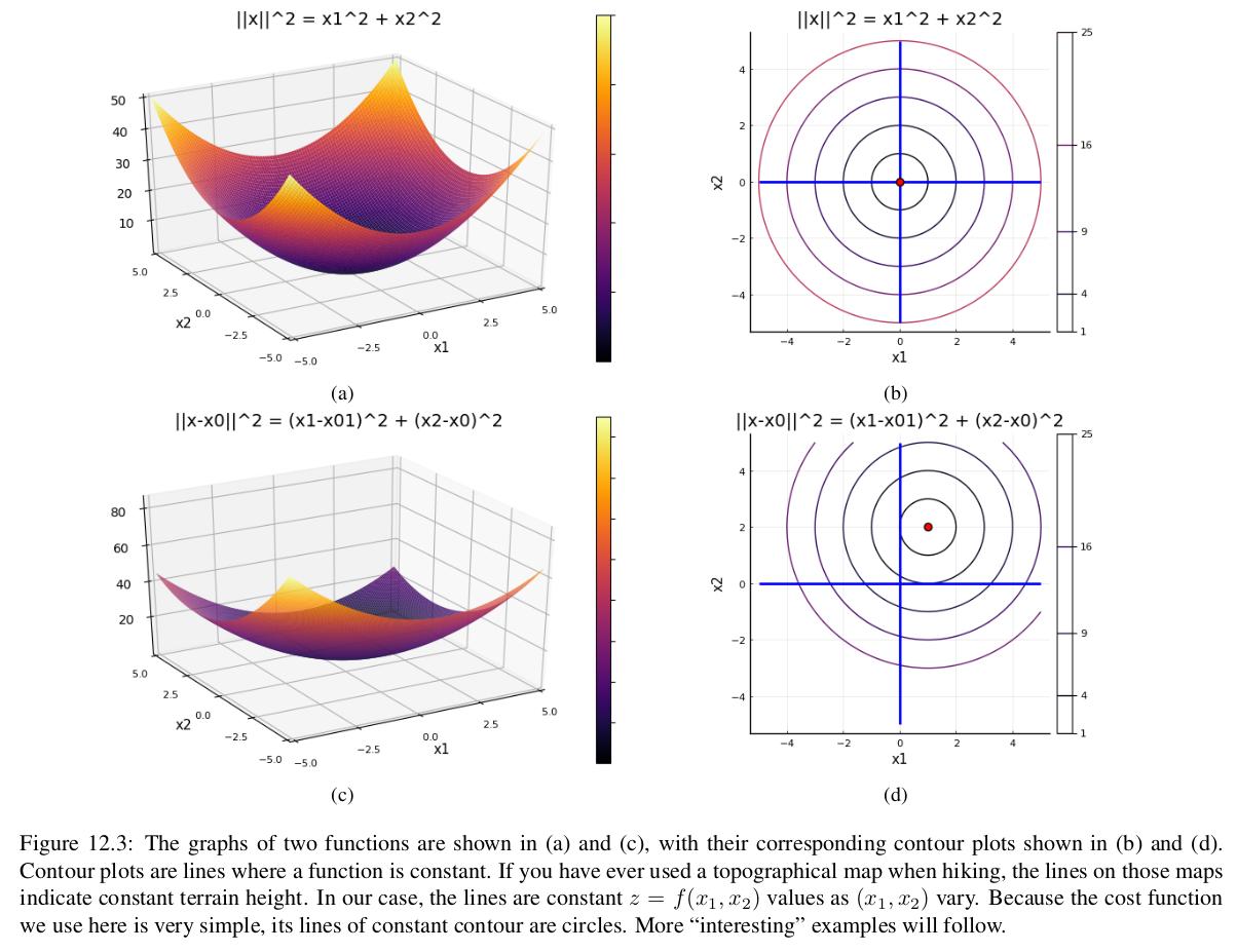
$f(\vv x) = \|\vv x\|^2 = x_1^2 + x_2^2$ , which is nothing but the Euclidean norm squared of $\vv x$ , and
$f(\vv x) = \|\vv x-\vv b\|^2 = (x_1-b_1)^2+(x_2-b_2)^2$ , which is a very simple least squares objective with $A=I$ .

We have plotted both of these functions, and their contour plots, below:

The contour plots show the level sets of $f(\vv x)$ , which we’ve seen before. These are the sets $C_{\alpha} = \{\vv x\in\mathbb{R}^2 | f(\vv x)=\alpha\}$ for some constant α. Here, these end up being circles, since for example $C_1$ is the set of $x_1,x_2$ such that $x_1^2 + x_2^2 = 1$ or $(x_1-b_1)^2 + (x_2-b_2)^2 = 1$ .

Can we use these contour plots to identify which way is down if our ant is currently sitting at point $\vv w\in\mathbb{R}^2$ ?

To answer this question, we’ll need the gradient $\nabla f(\vv x)$ of our function. Recall from Math 1410 that for a function $f:\mathbb{R}^n\to\mathbb{R}$ , its gradient $\nabla f(\vv x)$ is an n-vector of the partial derivatives of f:

\nabla f(\vv x) = \begin{bmatrix} \frac{\partial f}{\partial x_1}(\vv x) \\[6pt] \vdots \\[6pt] \frac{\partial f}{\partial x_n}(\vv x) \end{bmatrix} \in \mathbb{R}^n

(8)

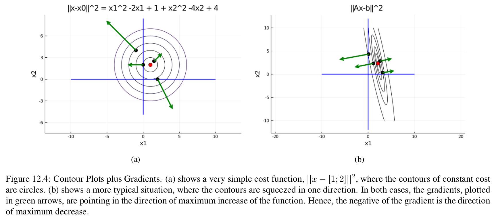
For our functions on $\mathbb{R}^2$ , this reduces to $\nabla f(\vv x) = \left(\frac{\partial f}{\partial x_1}(x_1, x_2), \frac{\partial f}{\partial x_2}(x_1, x_2)\right) \in \mathbb{R}^2$ .

In the figure below, we show contour plots for $f_1(\vv x)=\|\vv x-b\|^2=(x_1-1)^2+(x_2-2)^2$ and $f_2(x)=\|A\vv x-\vv b\|^2$ , along with the gradients $\nabla f(\vv x)$ (green arrows) at various points.

In both cases, the gradients are pointing in the direction of maximal increase: if we go in the opposite $-\nabla f(\vv x)$ direction, we will move in the direction of maximal decrease!

Let’s flex our calculus muscles a bit and compute the gradients of $f(\vv x)$ and $f_2(\vv x)$ ^[2]:

\nabla f_1(\vv x) = \begin{bmatrix} \frac{\partial}{\partial x_1}((x_1-1)^2+(x_2-2)^2) \\[6pt] \frac{\partial}{\partial x_2}((x_1-1)^2+(x_2-2)^2) \end{bmatrix} = 2\begin{bmatrix} x_1-1 \\[6pt] x_2-2 \end{bmatrix}

(9)

and

\nabla f_2(\vv x) = \nabla (A\vv x-\vv b)^T(A\vv x-\vv b) = 2A^T(A\vv x-\vv b)

(10)

One thing you might notice in the plots above is that the red dots, which we placed on the function minimum, have no green arrows. This is because the gradient at these points is zero. In fact, this is true in general: a point $\vv x$ is a local minimum only if $\nabla f(\vv x)=0$ .

We won’t prove this, but intuitively, this makes sense: if $\nabla f(\vv x)\neq \vv 0$ , then this means there is a direction $-\nabla f(\vv x)$ in which I could walk a little bit downhill to decrease $f(\vv x)$ , so $\nabla f(\vv x)$ must be zero if we’re at a local minima. Let’s check that this holds for $\nabla f_1(\vv x)$ and $\nabla f_2(\vv x)$ above:

For $f_1(\vv x)$ , $x^* = (1, 2)$ , and $\nabla f_1(\vv x^*) = 2\begin{bmatrix} x_1^*-1 \\ x_2^*-2 \end{bmatrix} = \vv 0$ , and so that checks out. And for $f_2(\vv x)$ , $\vv x^* = (A^TA)^{-1}A^T\vv b$ , and

$\nabla f_2(\vv x^*) = 2(A^TA \vv x^* - A^T\vv b) = 2\underbrace{(A^TA)(A^TA)^{-1}}_{I}(A^T\vv b - A^T\vv b) = 2(A^T\vv b - A^T\vv b) = \vv 0$ !

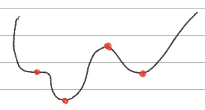
In general, while $\nabla f(\vv x^*) = \vv 0$ is necessary for $\vv x^*$ to be a local minima, it is not sufficient, i.e., there may be certain points with $\nabla f(\vv x^*)=\vv 0$ that are not local minima. For example, all red dots in the plot below have vanishing gradients, but only two are minima:

However, if our function $f$ is convex (bowl shaped), we have the following theorem which tells us that walking downhill will always find a global minimum:

Next, we’ll use our new found insights to define gradient descent, a widely used iterative algorithm for finding local minima of optimization problem (1).