5.2 Linear and Affine Transformations

1Reading¶

Material related to this page, as well as additional exercises, can be found in ALA 7.2 and 7.3.

2Learning Objectives¶

By the end of this page, you should know:

linear transformations and some examples
affine transformations
the transformation that preserves distance (isometry)

3Eucledian Linear Transformation¶

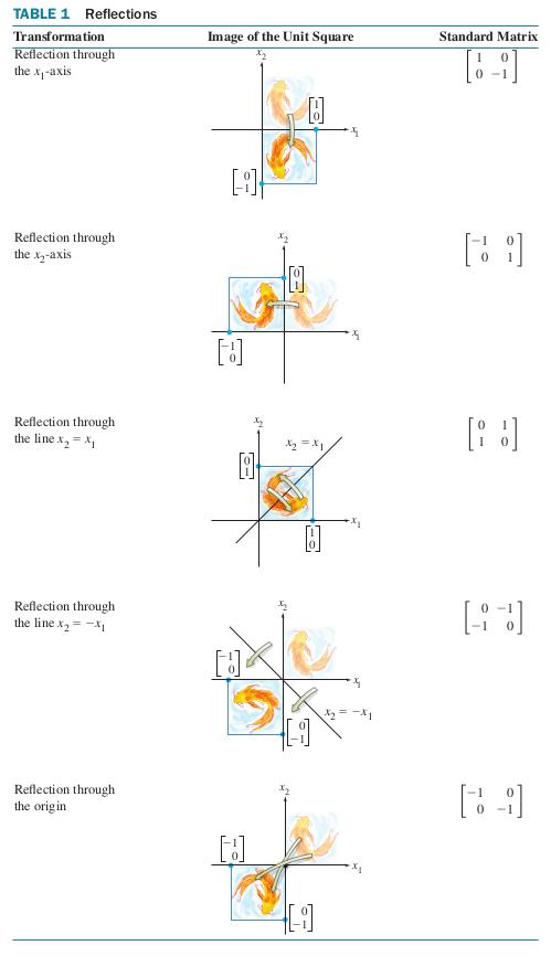
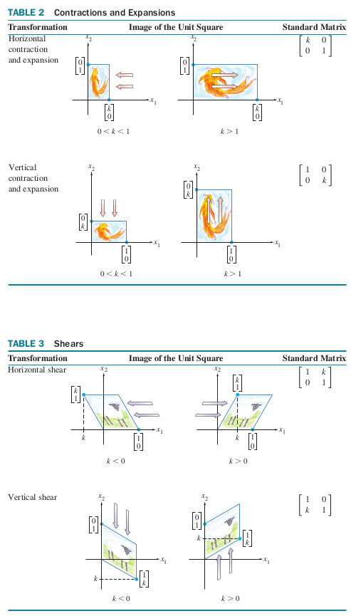
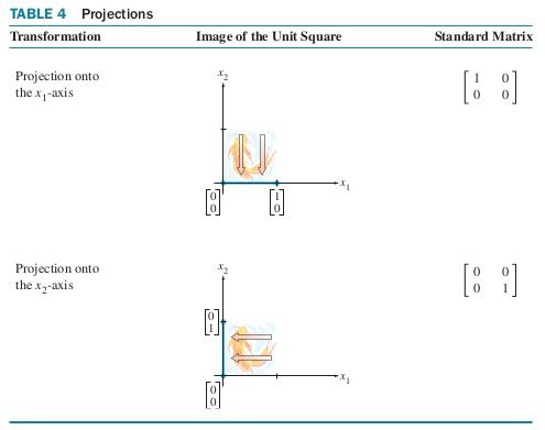
Functions that map $\mathbb{R}^n \to \mathbb{R}^n$ are called liner transformations. They are special cases of the more general linear transformations we saw in the previous section, but have a very nice geometric interpretation that help build intuition. In the tables below, we present some common trarsformatious of $\mathbb{R}^2$ , visualize their effect, and give their matrix representations.

4Affine Transformations¶

You will notice that translations are conspicuously missing from the examples we have seen so far. That’s because they are NOT linear functions! Rather, they are an example of slightly more general class of affine maps.

For example, a translation that translates a vector $\vv x$ can be written as $F (\vv x) = \vv x + \vv b$ , where $\vv b$ is the translation.

5Isometry¶

A key property of rigid motions (translations, rotations, reflections), which are ubiquitous in robotics, mechanics, and computer graphics, is that they are distance preserving. Informally, a transformation that preserves distance is known as an isometry. In the context of Euclidean spaces, this means that applying the linear transformation $A \vv x$ to a vector $\vv x$ does not change its norm, i.e., $\|A \vv x\| = \|\vv x\|$ .

We’ve argued informally that rotations and reflections are length-preserving. Let’s now make this precise.

To see that the translation $T(\vv x) = \vv x + \vv b$ satisfies this definition, note that

\begin{align*} \text{dist}(T(\vv x), T(\vv y)) &= \|T(\vv x) - T(\vv y)\| = \|(\vv x+ \vv b) - (\vv y+ \vv b)\| \\ &= \|\vv x - \vv y\| = \text{dist}(\vv x,\vv y). \end{align*}

(4)

5.1Move a Robot Manipulator and a Camera¶

The below animation shows a mobile manipulator that is viewed via a camera in first person view. The different configurations of the robot are shown by translation and rotation of the camera and the robot, all of which are linear transformations. If you are interested, you can run the block of code that is given after the animation on your local PC to actively interact with the camera and the robot as shown here. You will have to install PyBullet for running the code. PyBullet is a physics simulation engine used primarily for robotics applications.

import pybullet as p
import pybullet_data
import time

# Connect to PyBullet
physicsClient = p.connect(p.GUI)

# Set the search path to find the URDF files
p.setAdditionalSearchPath(pybullet_data.getDataPath())

# Load plane and mobile base
planeId = p.loadURDF("plane.urdf")
baseId = p.loadURDF("r2d2.urdf", basePosition=[0, 0, 0], useFixedBase=False)

# Load robotic arm and position it on top of the mobile base
robotId = p.loadURDF("kuka_iiwa/model.urdf", basePosition=[-0.1, 0, 0.4], useFixedBase=True)

# Set gravity
p.setGravity(0, 0, -9.8)

# Create sliders for camera control
camera_x = p.addUserDebugParameter("camera_x", -10, 10, 0)
camera_y = p.addUserDebugParameter("camera_y", -10, 10, 0)
camera_z = p.addUserDebugParameter("camera_z", -10, 10, 1)
camera_yaw = p.addUserDebugParameter("camera_yaw", -180, 180, 0)
camera_pitch = p.addUserDebugParameter("camera_pitch", -90, 90, -30)

# Create sliders for mobile base control
base_x = p.addUserDebugParameter("base_x", -10, 10, 0)
base_y = p.addUserDebugParameter("base_y", -10, 10, 0)
base_yaw = p.addUserDebugParameter("base_yaw", -180, 180, 0)

# Create sliders for robotic arm joints
joint_positions = []
num_joints = p.getNumJoints(robotId)
for i in range(num_joints):
    info = p.getJointInfo(robotId, i)
    joint_positions.append(p.addUserDebugParameter(f'Joint {info[1].decode("utf-8")}', -3.14, 3.14, 0))

# Main loop
while True:
    # Read camera parameters
    cam_x = p.readUserDebugParameter(camera_x)
    cam_y = p.readUserDebugParameter(camera_y)
    cam_z = p.readUserDebugParameter(camera_z)
    cam_yaw = p.readUserDebugParameter(camera_yaw)
    cam_pitch = p.readUserDebugParameter(camera_pitch)
    
    # Set the camera position and orientation
    p.resetDebugVisualizerCamera(cameraDistance=2, cameraYaw=cam_yaw, cameraPitch=cam_pitch, cameraTargetPosition=[cam_x, cam_y, cam_z])
    
    # Read base parameters
    base_x_pos = p.readUserDebugParameter(base_x)
    base_y_pos = p.readUserDebugParameter(base_y)
    base_yaw_angle = p.readUserDebugParameter(base_yaw)
    
    # Set the base position and orientation
    p.resetBasePositionAndOrientation(baseId, [base_x_pos, base_y_pos, 0], p.getQuaternionFromEuler([0, 0, base_yaw_angle]))
    
    # Get base orientation and position
    base_position, base_orientation = p.getBasePositionAndOrientation(baseId)
    
    # Compute the new position for the robot arm
    new_robot_position = [base_position[0]-0.1, base_position[1], base_position[2] + 0.4]
    
    # Set the new position and orientation for the robot arm
    p.resetBasePositionAndOrientation(robotId, new_robot_position, base_orientation)

    # Read and set robotic arm joint positions
    for i in range(num_joints):
        joint_position = p.readUserDebugParameter(joint_positions[i])
        p.setJointMotorControl2(bodyUniqueId=robotId, jointIndex=i, controlMode=p.POSITION_CONTROL, targetPosition=joint_position)
    
    # Step the simulation
    p.stepSimulation()
    
    # Sleep for a while to slow down the simulation
    time.sleep(0.01)

# Disconnect from PyBullet
p.disconnect()

pybullet build time: Oct 14 2023 15:44:17

6Linear Operators and Linear Systems (Optional Advanced Material)¶

Here we briefly highlight the generality of the machinery we’ve developed so far by dipping our toes into the world of linear operators. A linear operator is a linear transformation mapping between function spaces.

We’ll look at one particular class of linear operators, called differential operators, as they lie at the heart of differential equations, which we will be studying next.

We will work with the following function spaces:

$C^0[0,1]$ , the space of continuous functions defined on the interval $[0,1]$ ; and
$C^1[0,1]$ , the space of continuously differentiable functions over the interval $[0,1]$