8.1 Linear Iterative Systems

1Reading¶

Material related to this page, as well as additional exercises, can be found in ALA 9.1.

2Learning Objectives¶

By the end of this page, you should know:

the stable behavior of discrete time scalar system
the definition of a general linear iterative system
the general solution to linear iterative systems using eigenvectors
how to compute the general solution using diagonalization and iteration

3Discrete Time System¶

So far, we have focused on continuous time dynamical systems, for which the time index $t$ of the solution $\vv x(t)$ is continuous, i.e., $t \in \mathbb{R}$ . This is a natural model to use for many systems, such as for example those evolving according to the laws of physics. However, in other instances, it is more natural to consider time in discrete steps. For example, when banks add interest to a savings account, they typically do so on a monthly or yearly basis. More specifically, suppose at period $k$ , we have $x(k)$ dollars in our account, and an interest rate of $r$ is applied. Then $x(k+1) = (1+r)x(k)$ . This defines a scalar linear iterative system, whichtake the general form

x(k+1) = \lambda x(k), \quad x(0) = a.

(1)

If we roll out the dynamics (1), we easily compute:

\begin{align*} x(0) &= a, \\ x(1) &= \lambda a, \\ x(2) &= \lambda^2 a, \\ &\ldots \\ x(k) &= \lambda^k a \quad \text{for any positive integer } k. \end{align*}

(2)

We therefore immediately conclude that there are three possibilities for $x(0) = a \neq 0$ :

Stable: If $|\lambda| < 1$ , then $|x(k)| \to 0$ as $k \to \infty$
Marginally Stable: If $|\lambda| = 1$ , then $|x(k)| = |a|$ for all $k \in \mathbb{N}$ , where $\mathbb{N} = \{0, 1, 2, \ldots, \ldots \}$ (non-negative integers)
Unstable: If $|\lambda| > 1$ , then $|x(k)| \to \infty$ as $k \to \infty$

Our goal is to extend this analysis to the general linear iterative systems, that is formally defined below.

We will then use these tools to study a very important class of linear iterative systems called Markov Chains, which can be used for everything from internet search (Google’s search algorithm PageRank) to baseball statistics (DraftKings uses these ideas to set betting odds!).

4Powers of Matrices¶

Rolling out the dynamics (3), we again see a clear solution to (3):

\begin{align*} \vv x(0) &= \vv a, \\ \vv x(1) &= T \vv a, \\ \vv x(2) &= T^2 \vv a, \\ &\ldots \\ \vv x(k) &= T^k \vv a \quad \text{for all } k \in \mathbb{N}. \end{align*}

(4)

However, unlike the scalar setting (1), the qualitative behavior of $\vv x(k) = T^k \vv a$ as $k \to \infty$ is much less obvious. Since the scalar solution $x(k) = \lambda^k a$ is defined in terms of powers of λ, let’s try a similar guess for the vector-valued setting: $\vv x(k) = \lambda^k \vv v$ . Under what conditions on λ and $\vv v$ is $\vv x(k) = \lambda^k \vv v$ a solution to (3)? On one hand, we have that $\vv x(k+1) = \lambda^{k+1} \vv v$ . On the other, we have

T\vv x(k) = T(\lambda^k \vv v) = \lambda^k T\vv v.

(5)

The expressions $\vv x(k+1) = \lambda^{k+1} \vv v$ and $T\vv x(k) = \lambda^k T\vv v$ will be equal if and only if $T \vv v = \lambda \vv v$ , i.e., if and only if $(\lambda, \vv v)$ is an eigenvalue/vector pair of $T$ .

Thus, for each eigenvalue/vector pair $(\lambda_i, \vv v_i)$ of $T$ , we can construct a solution $\vv x_i(k) = \lambda_i^k \vv v_i$ to (3). By linear superposition, we can use this observation to characterize all solutions for complete matrices.

Theorem 1 (The solution to a linear iterative system with complete coefficient matrix)

If the coefficient matrix $T$ is complete (i.e., diagonalizable), then the general solution to the linear iterative system $\vv x(k+1) = T\vv x(k)$ is given by

\vv x(k) = c_1 \lambda_1^k \vv v_1 + c_2 \lambda_2^k \vv v_2 + \cdots + c_n \lambda_n^k \vv v_n,

(6)

where $\vv v_1, \ldots, \vv v_n$ are linearly independent eigenvectors of $T$ with corresponding eigenvalues $\lambda_1, \ldots, \lambda_n$ , and coefficients $c_1, \ldots, c_n$ are scalars uniquely prescribed by the initial condition

\vv x(0) = \bm \vv v_1 & \vv v_2 & \cdots & \vv v_n \em \vv c = \vv a.

(7)

We can extend this theorem to incomplete matrices using Jordan Blocks, but the idea remains the same.

Example 1

Consider the iterative system $\vv x(k+1) = T\vv x(k)$ defined by

\bm x_1(k+1) \\ x_2(k+1) \em = \bm .6 & .2 \\ .2 & .6 \end{bmatrix} \bm x_1(k) \\ x_2(k) \em, \quad \bm x_1(0) \\ x_2(0) \em = \bm a_1 \\ a_2 \em.

(8)

$T$ has eigenvalue/vector pairs:

\lambda_1 = .8, \ \vv v_1 = \begin{bmatrix} 1 \\ 1 \end{bmatrix} \quad \text{and} \quad \lambda_2 = .4, \; \vv v_2 = \begin{bmatrix} -1 \\ 1 \end{bmatrix}.

(9)

Therefore, the eigensolutions are

\vv x_1(k) = \lambda_1^k \vv v_1 = (.8)^k \begin{bmatrix} 1 \\ 1 \end{bmatrix} \quad \text{and} \quad \vv x_2(k) = \lambda_2^k \vv v_2 = (.4)^k \begin{bmatrix} -1 \\ 1 \end{bmatrix}.

(10)

Thus, a general solution is given by

\vv x(k) = c_1 \vv x_1(k) + c_2 \vv x_2(k) = c_1(.8)^k \begin{bmatrix} 1 \\ 1 \end{bmatrix} + c_2(.4)^k \begin{bmatrix} -1 \\ 1 \end{bmatrix}

(11)

To determine $c_1$ and $c_2$ , we solve

\vv x(0) = \begin{bmatrix} c_1 - c_2 \\ c_1 + c_2 \end{bmatrix} = \begin{bmatrix} a_1 \\ a_2 \end{bmatrix} \Rightarrow c_1 = \frac{a_1+a_2}{2}, \ c_2 = \frac{a_2-a_1}{2}

(12)

giving the specific solution

\bm x_1(k) \\ x_2(k) \em = \frac{a_1 + a_2}{2}(.8)^k \bm 1 \\ 1 \em + \frac{a_2 - a_1}{2}(.4)^k \bm -1 \\ 1 \em.

(13)

We conclude that $\vv x(k) \to 0$ as $k \to \infty$ , and that the slowest decaying direction is $\vv v_1 = \begin{bmatrix} 1 \\ 1 \end{bmatrix}$ , which decays at rate 0.8 (gets 20% smaller) each time step. We can visualize this in the plot below; we sampled initial conditions along the unit circle (shown in orange) and plotted the iterates after 0, 1, 2, 3, 4 (corresponding to orange, green, blue, purple, red respectively) time steps.

Example 2 (Solving a

3\times 3

linear iterative system (ALA Example 9.7))

Let $T = \bm -3&1&6\\1&-1&-2\\-1&-1&0\em$ be the coefficient matrix for a three-dimensional iterative system $\vv{u}(k + 1) = T\vv u(k)$ . Its eigenvalues and corresponding eigenvectors are

\begin{array}{ccc} \lambda_1 = -2, & \lambda_2 = -1 + i, & \lambda_3 = -1 -i,\\ \vv{v_1} = \bm 4\\-2\\1\em, & \vv{v_2} = \bm 2 - i \\ -1 \\ 1 \em, & \vv{v_3} = \bm 2 + i \\ -1 \\ 1\em. \end{array}

(14)

These eigenvectors are linearly independent and hence $T$ is complete. Applying the above result on linear iterative systems with complete coefficient matrices, the general complex solution to this is

\vv{u}(k) = v_1(-2)^k \bm 4\\-2\\1\em + b_2 (-1 + i)^k\bm 2-i\\-1\\1\em + b_3 (-1 - i)^k\bm 2 + i\\-1\\1\em

(15)

where $b_1, b_2, b_3$ are complex scalars corresponding to the choice of initial condition $\vv u(0)$ .

If we are only interested in real solutions (e.g., if the initial conditions are real), we can break up any complex solution into its real and imaginary parts, each of which constitutes a real solution. We begin by writing $\lambda_2 = -1 + i = \sqrt 2 (\cos{\frac 3 4 \pi} + i\sin{\frac 3 4 \pi}) = \sqrt 2 e^{3\pi i/4}$ in polar form, and hence (applying Euler’s formula),

(-1 + i)^k = (\sqrt 2) ^ke^{\frac 3 4 k\pi i} = (\sqrt 2) ^k (\cos {\frac 3 4 k \pi} + i \sin {\frac 3 4 k \pi}).

(16)

Therefore, the complex solution corresponding to $\lambda_2 = -1 + i$ can be rewritten as

(-1 + i)^k\bm 2 - i\\ -1\\1\em = (\sqrt 2)^k \bm 2\cos {\frac 3 4 k \pi} + \sin {\frac 3 4 k \pi} \\ -\cos {\frac 3 4 k \pi} \\ \cos{\frac 3 4 k \pi}\em + i (\sqrt 2)^k \bm 2\sin{\frac 3 4 k \pi} - \cos{\frac 3 4 k \pi} \\ -\sin {\frac 3 4 k \pi} \\ \sin{\frac 3 4 k\pi} \em

(17)

can be rewritten as a (complex) combination of two linearly independent real solutions! We do the same for the complex conjugate eigenvalue $\lambda_3 = -1 -i$ , which leads to the complex conjugate solution and the same two real solutions:

(-1 - i)^k\bm 2 + i\\ -1\\1\em = (\sqrt 2)^k \bm 2\cos{\frac 3 4 k \pi} + \sin{\frac 3 4 k \pi}\\-\cos{\frac 3 4 k \pi} \\ \cos{\frac 3 4 k \pi} \em - i (\sqrt 2)^k \bm 2\sin{\frac 3 4 k \pi} - \cos{\frac 3 4 k \pi} \\ -\sin {\frac 3 4 k \pi} \\ \sin{\frac 3 4 k\pi} \em

(18)

Note that this is incredibly similar to our approach for rewriting complex solutions to linear ODEs! We take the complex base solutions, and use Euler’s identity to rewrite them as (complex) linear combinations of real solutions! Thus, the general real solution $\vv{u}(k)$ to the system can be written as a linear combination of the three independent real solutions:

c_1 (-2)^k \bm 4\\-2\\1\em + c_2 (\sqrt 2)^k \bm 2\cos {\frac 3 4 k \pi} + \sin {\frac 3 4 k \pi} \\ -\cos {\frac 3 4 k \pi} \\ \cos{\frac 3 4 k \pi}\em + c_3 (\sqrt 2)^k \bm 2\sin{\frac 3 4 k \pi} - \cos{\frac 3 4 k \pi} \\ -\sin {\frac 3 4 k \pi} \\ \sin{\frac 3 4 k\pi} \em

(19)

where $c_1, c_2, c_3$ are arbitrary real scalars (assuming that the initial conditions are real), uniquely prescribed by the initial conditions.

4.1Python break!¶

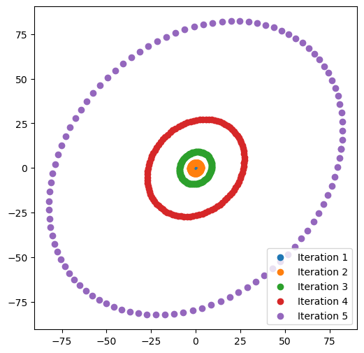
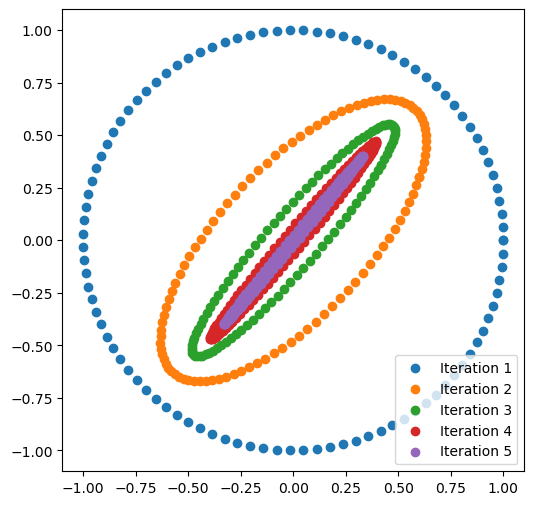
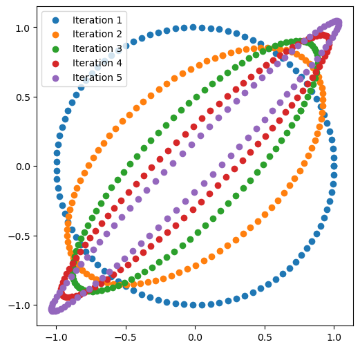
In the below python code, we solve different linear iterative systems by computing the eigen values and eigen vectors of the coefficient matrix. We plot the results of the iterates as in Figure 1, where the initial conditions are sampled from the unit circle and observe the different behaviors for each coefficient matrix.

import numpy as np
import matplotlib.pyplot as plt

def plot_iterates(T):
    
    eigvals, eigvecs = np.linalg.eig(T)
    
    print("Eigen Values: ", eigvals)
    
    # Initial conditions on the unit circle
    theta = np.linspace(0, 2*np.pi, 100)    
    init = np.vstack((np.cos(theta).reshape((1,-1)), np.sin(theta).reshape((1,-1)))) 
    
    c = np.linalg.solve(eigvecs, init) # solving for the c vector using the initial conditions
    
    x_all = []
    T = 5
    
    plt.figure(figsize=(8, 6))
    
    labels = [f'Iteration {i + 1}' for i in range(T)]
    for i in range(T):
        x_t = (eigvals**i * eigvecs) @ c
        x_all.append(x_t)
        plt.scatter(x_t[0, :], x_t[1, :], label=labels[i])
    plt.legend()
    plt.gca().set_aspect('equal')
    plt.show()

# Notice the difference between the plots and the corresponding eigen values    
T = np.array([[3, .1], [.1, 3]])
plot_iterates(T)
T1 = np.array([[.6, .2], [.3, .6]])
plot_iterates(T1)
T2 = np.array([[.2, .9], [.8, .3]])
plot_iterates(T2)

Eigen Values:  [3.1 2.9]

Eigen Values:  [0.84494897 0.35505103]

Eigen Values:  [-0.6  1.1]

5Diagonalization and Iteration¶

An alternative and equally efficient approach to solving (3) in the case of complex matrices is based on the diagonalization of T. We start with the following observation (which we also saw when computing the matrix exponential). Let $V = \bm \vv v_1 & \cdots & \vv v_n\em$ be an eigenbasis for $T$ , and $\Lambda = \text{diag}(\lambda_1, \ldots, \lambda_n)$ the diagonal matrix of the eigenvalues of $T$ . Then:

\begin{align*} T &= V \Lambda V^{-1} \\ T^2 &= V \Lambda V^{-1} V \Lambda V^{-1} = V \Lambda^2 V^{-1} \\ T^3 &= T(T^2) = V \Lambda V^{-1} V \Lambda^2 V^{-1} = V \Lambda^3 V^{-1} \end{align*}

(20)

and in general, $T^k = V \Lambda^k V^{-1}$ . Therefore, the solution to $\vv x(k+1) = T\vv x(k)$ , with $\vv x(0) = \vv a$ is

\vv x(k) = T^k \vv a = V \Lambda^k V^{-1} \vv a.

(21)

If we define $\vv c = V^{-1}\vv a$ , then we recover $\vv x(k) = c_1 \lambda_1^k \vv v_1 + \cdots + c_n \lambda_n^k \vv v_n$ .

Example 3 (Solving a

2\times 2

linear iterative system with diagonalization)

Let $T = \bm 7&6\\-9&-8\em$ . Its eigenvalues and eigenvectors are:

\lambda_1 = -2, \quad \vv{v_1} = \bm -2\\3\em, \qquad \lambda_2 = 1, \quad \vv{v_2} = \bm -1\\1\em.

(22)

We assemble these into the diagonal eigenvalue matrix $S$ and the eigenvector matrix $P$ , given by

D = \bm -2 &0\\0&1\em, \qquad P = \bm -2&-1\\3&1\em,

(23)

such that a diagonalization of $T$ is given by $T = PDP^{-1}$ . Therefore, using the results above,

\begin{align*} T^k = PD^kP^{-1} &= \bm -2&-1\\3&1\em \bm (-2)^k &0\\0&1 \em \bm 1&1\\-3&-2\em\\ &= \bm 3-2(-2)^k & 2 -2(-2)^k\\-3 + 3(-2)^k&-2 + 3(-2)^k \em. \end{align*}

(24)

It follows that the solution to the particular iterative system with coefficient matrix $T$ and initial conditions $\vv u(0)$ is given by

\vv u(k) = T^k \vv u(0) = \bm 3-2(-2)^k & 2 -2(-2)^k\\-3 + 3(-2)^k&-2 + 3(-2)^k \em\vv u(0).

(25)

5.1Python break!¶

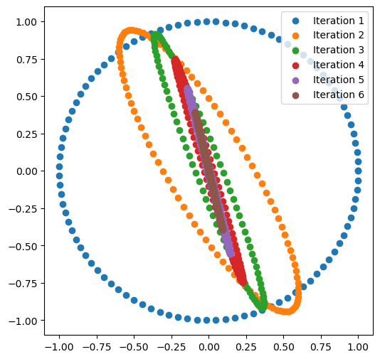
In the below python script, we diagonalize the coefficient matrix and plot the solution at different iterates. This method eliminates the need to solve for the c vector as in Example 1, but we can directly solve the system using the initial conditions and the diagonalization as in Example 3.

# given a square matrix A, returns a tuple of matrices (P, D) such that A = PDP^{-1}
def diagonalize(A):
    evals, evecs = np.linalg.eig(A)
    print("Eigen Values: ", evals)
    return evecs, np.diag(evals)

def plot_iterates(P, D):
    # Initial conditions on the unit circle
    theta = np.linspace(0, 2*np.pi, 100)    
    init = np.vstack((np.cos(theta).reshape((1,-1)), np.sin(theta).reshape((1,-1))))
    # Plot initial conditions
    x_all = [init]
    T = 5
    labels = [f'Iteration {i + 1}' for i in range(T+1)]    
    plt.figure(figsize=(8, 6))
    plt.scatter(init[0, :], init[1, :], label=labels[0])

    # Iterates
    for i in range(1, T+1):
        Ti = P @ D**i @ np.linalg.inv(P)
        x_i = Ti @ init
        x_all.append(x_i)
        plt.scatter(x_i[0, :], x_i[1, :], label=labels[i])
    plt.legend()
    plt.gca().set_aspect('equal')
    plt.show()

T2 = np.array([[-0.6, 0.01], [0.8, -0.5]])
P, D = diagonalize(T2)
plot_iterates(P, D)

Eigen Values:  [-0.65246951 -0.44753049]