11.1 Basics of Statistics

1Reading¶

Material related to this page, as well as additional exercises, can be found in LAA 7.5 and ALA 8.8.

2Learning Objectives¶

By the end of this page, you should know:

the idea of studying only important features of an image
what is an observation matrix
the sample mean and covariance of observations with some examples

3Motivation: Satellite Imagery¶

We start with a motivating application from satellite imagery analysis. The Landsat satellites are a pair of imaging satellites that record images of terrain and coastlines. These satellites cover almost every square mile of the Earth’s surface every 16 days.

Satellite sensors acquire seven simultaneous images of any given region, with each sensor recording energy from separate wavelength bands: three in the visible light spectrum and four in the infrared and thermal bands.

Each image is digitized and stored as a rectangular array of numbers, with each number representing the signal intensity at the corresponding pixel. Each of the seven images is one channel of a multichannel or multispectral image.

The seven Landsat images of a given region typically contain a lot of redundant information, as some features will appear across most channels. However, other features, because of their color or temperature, may only appear in one or two channels. A goal of multispectral image processing is to view the data in a way that extracts information better than studying each image separately.

One approach, called Principal Component Analysis (PCA), seeks to find a special linear combination of the data that takes a weighted combination of all seven images into just one or two images. Importantly, we want these one or two composite images. or principal components to capture as much of the scene variance (features) as possible; in particular, features should be more visible in the composite images than any of the original individual ones.

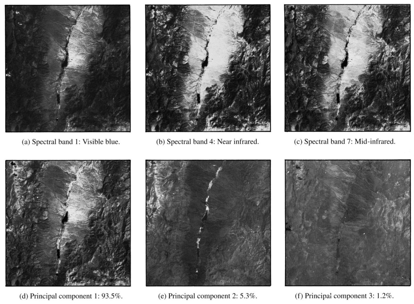
This idea, which we’ll explore in detail today, is illustrated with some Landsat imagery taken over Railroad Valley Nevada.

Images from three Landsat spectral bands are shown in (a)-(c); the total information in these images is “rearranged” into the three principal components in (d)-(f). The first component, (d), “explains” 93.5% of the scene features (or variance) found in the original data. In this way, we could compress all of the original data to the single image (d) with only a 6.5% loss of scene variance.

PCA can in general be applied to any data that consists of lists of measurements made on a collection of objects or individuals, including data mining, machine learning, image processing, speech recognition, facial recognition, and health informatics. As we’ll see next, the way in which these “special combinations” of measurements are computed are via the singular vectors of an observation matrix.

4Observation Matrix¶

Let $\mathbf{x}_j \in \mathbb{R}^p$ denote an observation vector obtained from measurement $j$ , and suppose that $j=1,\ldots,N$ measurements are obtained. The observation matrix $X \in \mathbb{R}^{p \times N}$ is a $p \times N$ matrix with $j^{th}$ column equal to the $j^{th}$ measurement vector $\mathbf{x}_j$ :

X = \bm \mathbf{x}_1 & \mathbf{x}_2 & \cdots & \mathbf{x}_N\em \in \mathbb{R}^{p \times N}

(1)

5Mean and Covariance¶

To understand PCA, we need to understand some basic concepts from statistics. We will review the mean and covariance of a set of observations $\vv x_1, \ldots, \vv x_N$ . For our purposes, these will simply be things we can compute from the data, but you should be aware that these are well motivated quantities from a statistical perspective.: you will learn more about this in ESE 3010, STAT 4300 or ESE 4020.

Let’s start with an observation matrix $X \in \mathbb{R}^{p\times N}$ , with columns $\mathbf{x}_1,\ldots,\mathbf{x}_N \in \mathbb{R}^p$ .

Since PCA is interested in directions of (maximal) variation in our data, it makes sense to subtract off the mean $\mathbf{m}$ , as it captures the average behavior of our data set. To that end, define the centered observations to be

\hat{\mathbf{x}}_j = \mathbf{x}_j - \mathbf{m}, \quad j=1,\ldots,N,

(4)

and the centered or de-meaned observation matrix

\hat{X} = \bm \hat{\mathbf{x}}_1 & \hat{\mathbf{x}}_2 & \cdots & \hat{\mathbf{x}}_N\em.

(5)

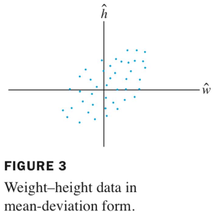
For example, Fig. 3 below shows a centered version of the weight/height data illustrated in Fig. 1:

Since any matrix of the form $AA^T$ is positive semidefinite (can you see why?), so is $S$ . Note sometimes $\frac{1}{N-1}$ is used as normalization; this is motivated for statistical considerations beyond the scope of this course (it leads to $S$ being an unbiased estimator of the “true” covariance of the data). We will just use $\frac{1}{N}$ .

Example 3

Three measurements are made on each of four individuals in a random sample from a population. The observation vectors are:

\mathbf{x}_1 = \begin{bmatrix} 1 \\ 2 \\ 1 \end{bmatrix}, \quad \mathbf{x}_2 = \begin{bmatrix} 4 \\ 2 \\ 13 \end{bmatrix}, \quad \mathbf{x}_3 = \begin{bmatrix} 7 \\ 8 \\ 1 \end{bmatrix}, \quad \mathbf{x}_4 = \begin{bmatrix} 8 \\ 4 \\ 5 \end{bmatrix}

(7)

The sample mean is $\mathbf{m} = \frac{1}{4}\left(\mathbf{x}_1+\mathbf{x}_2+\mathbf{x}_3+\mathbf{x}_4\right) = \begin{pmatrix} 5 \\ 4 \\ 5 \end{pmatrix}$ .

The centered observations $\hat{\mathbf{x}}_j = \mathbf{x}_j - \mathbf{m}$ are then

\hat{\mathbf{x}}_1 = \begin{bmatrix} -4 \\ -2 \\ -4 \end{bmatrix}, \quad \hat{\mathbf{x}}_2 = \begin{bmatrix} -1 \\ -2 \\ 8 \end{bmatrix}, \quad \hat{\mathbf{x}}_3 = \begin{bmatrix} 2 \\ 4 \\ -4 \end{bmatrix}, \quad \hat{\mathbf{x}}_4 = \begin{bmatrix} 3 \\ 0 \\ 0 \end{bmatrix},

(8)

and the centered observation matrix is

\hat{X} =\begin{bmatrix} -4 & -1 & 2 & 3 \\ -2 & -2 & 4 & 0 \\ -4 & 8 & -4 & 0 \end{bmatrix}.

(9)

The sample covariance matrix is

S = \frac{1}{4} \hat{X}\hat{X}^T = \begin{bmatrix} 7.5 & 4.5 & 0 \\ 4.5 & 6 & -6 \\ 0 & -6 & 24 \end{bmatrix}.

(10)

You might be wondering what the entries $s_{ij}$ of the covariance matrix $S$ mean. Let’s take a bit of a closer look. We’ll consider a small example where the observations $\mathbf{x}_j \in \mathbb{R}^2$ are two dimensional, and assume we have $N=3$ observations. Let the first measurement be $a \in \mathbb{R}$ and the second $b \in \mathbb{R}$ , so that $\mathbf{x}_i = (a_i, b_i) \in \mathbb{R}^2$ and the centered observation is $\hat{\mathbf{x}}_i = (\hat{a}_i, \hat{b}_i) \in \mathbb{R}^2$ . Our centered observation matrix is then

\hat{X} = \bm \hat{a}_1 & \hat{a}_2 & \hat{a}_3 \\ \hat{b}_1 & \hat{b}_2 & \hat{b}_3 \em = \bm \hat{\mathbf{a}}^T \\ \hat{\mathbf{b}}^T \em,

(11)

where we defined $\hat{\mathbf{a}} = (\hat{a}_1, \hat{a}_2, \hat{a}_3) \in \mathbb{R}^3$ and $\hat{\mathbf{b}} = (\hat{b}_1, \hat{b}_2, \hat{b}_3)$ as the vectors in $\mathbb{R}^3$ containing all of the centered first and second measurements, respectively.

Then, we can write our sample covariance matrix as:

S = \frac{1}{3} \hat{X}\hat{X}^T = \frac{1}{3} \bm \hat{\mathbf{a}}^T \\ \hat{\mathbf{b}}^T \em \bm \hat{\mathbf{a}} & \hat{\mathbf{b}} \em = \begin{bmatrix} \frac{\|\hat{\mathbf{a}}\|^2}{3} & \frac{\hat{\mathbf{a}}^T\hat{\mathbf{b}}}{3} \\ \frac{\hat{\mathbf{a}}^T\hat{\mathbf{b}}}{3} & \frac{\|\hat{\mathbf{b}}\|^2}{3} \end{bmatrix}.

(12)

The diagonal entry $s_{11} = \frac{\|\hat{\mathbf{a}}\|^2}{3}$ is called the variance of measurement 1.

Expanding it out:

\begin{align*} s_{11} = \frac{\|\hat{\mathbf{a}}\|^2}{3} &= \frac{1}{3}(\hat{a}_1^2 + \hat{a}_2^2 + \hat{a}_3^2) \\ &= \frac{1}{3}((a_1-m_1)^2 + (a_2-m_2)^2 + (a_3-m_3)^2) \end{align*}

(13)

we see that $s_{11}$ captures how much the first measurement $a_i$ deviates from its mean value $m_i$ , on average, i.e., it measures how much $a_i$ varies relative to its mean. Similarly, $s_{22} = \frac{\|\hat{\mathbf{b}}\|^2}{3}$ is the variance of measurement 2.

Now let’s look at the off-diagonal term $s_{12} = s_{21} = \frac{\hat{\mathbf{a}}^T\hat{\mathbf{b}}}{3}$ . Recall from our work on inner products that $\hat{\mathbf{a}}^T\hat{\mathbf{b}} = \|\hat{\mathbf{a}}\| \|\hat{\mathbf{b}}\| \cos \theta$ , where θ is the angle between $\hat{\mathbf{a}}$ and $\hat{\mathbf{b}}$ . We can view

\cos \theta = \frac{\hat{\mathbf{a}}^T\hat{\mathbf{b}}}{\|\hat{\mathbf{a}}\| \|\hat{\mathbf{b}}\|}

(14)

as a measure of how well aligned, or correlated: if $\hat{\mathbf{a}}$ and $\hat{\mathbf{b}}$ are parallel, $\cos \theta = 1$ or -1, and if $\hat{\mathbf{a}}$ and $\hat{\mathbf{b}}$ are perpendicular, $\cos \theta = 0$ . This lets us interpret $s_{12} = \frac{\hat{\mathbf{a}}^T\hat{\mathbf{b}}}{3}$ , which is proportional to $\cos \theta$ , as a measure of how similarly $\hat{\mathbf{a}}$ and $\hat{\mathbf{b}}$ deviate from their means: if $\hat{\mathbf{a}}^T\hat{\mathbf{b}}$ is positive, this means $\hat{\mathbf{a}}$ and $\hat{\mathbf{b}}$ tend to move up or down together; if it is negative they tend to move in opposite directions; and if it is small (or zero), $\hat{\mathbf{a}}$ and $\hat{\mathbf{b}}$ tend to move independently of each other. Since $s_{12}$ captures how the 1st and 2nd measurements vary with each other, it is called their covariance.

Finally, although we worked out the concepts for $\vv x_j \in \mathbb{R}^p$ and $j=1,2,3,$ These concepts extend naturally to the general setting:

$S_{ii}$ = variance of measurement $i$ across measurements $j=1,\ldots,N$
$S_{kl}$ = cvariance of measurements $k$ and $l$ across measurements $j=1,\ldots,N$ .