2.7 Case Study: Network Flows Revisited

Lecture notes

1Reading¶

Material related to this page, as well as additional exercises, can be found in ALA Ch. 1.6.

2Learning Objectives¶

By the end of this page, you should know:

• how to represent flows in networks as matrices
• the sources and sinks in a network
• the relationship of flow conservation to linear systems

3Incidence Matrix¶

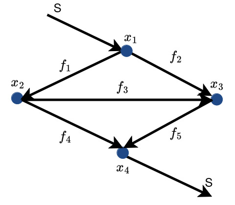
Consider the directed graph below with 4 nodes and 5 edges

We can associate an incidence matrix $A$ with this graph. Each row corresponds to a node, and each column to an edge, with

For Figure 1, $A \in \mathbb{R}^{4 \times 5}$, and

By considering the four fundamental subspaces (Row, Column, Null and Left Null Space) of $A$, we can completely understand the properties of our network flow problem. The incidence flow can be represented in code using numpy as follows:

4The Current Law¶

First, we define the source vector $\vv s = \bm s \\ 0 \\ 0 \\ -s \em$, which captures external flows entering (positive entries) the network referred to as sources, and flows leaving (negative entries) the network known as sinks. We make sure $\vv 1^{\top} \vv s = 0$.

The flow conservation equations say that flows entering a node must equal flows leaving a node, which can be written as

where $\vv f = \bm f_1 \\ f_2 \\ f_3 \\ f_4 \\ f_5 \em \in \mathbb{R}^{5}$ is the vector of edge flows. The solution set to (3) characterizes all flows compatible with the network and the source vector $\vv s$.

From this theorem, we see that $A \vv f = - \vv s$ has a solution if and only if $\vv s \in$Col$(A)$. Let’s try to understand when this might be true by computing a basis for Col$(A)$.

From (2), we notice that

1. columns 1, 2 and 3 are not independent: column 3 = column 2 - column 1.
2. columns 3, 4 and 5 are not independent: column 5 = column 4 - column 3 = column 4 - column2 + column 1

However, we have that columns 1, 2 and 4 are independent! Since we can represent columns 3 and 5 in terms of columns 1, 2 and 4; columns 1, 2 and 4 span Col$(A)$. We conclude that columns 1, 2 and 4 form a basis for Col$(A)$, and dim(Col$(A)) = 3$.

Now, let’s take a closer look at Figure 1: edges $1, 2$ and 3 form a loop in the graph, while edges $3, 4$ and 5 form another loop. In contrast, edges $1, 2$ and 4 form a tree, which has no loops! This tells us that the edges of any tree in our graph gives us independent columns!

So we now check if $\vv s \in$Col$(A)$ using columns $1, 2$ and 4.

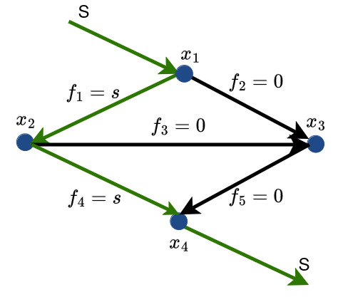
which has solution $f_1 = f_4 = s$ and $f_2 = 0$. Therefore, one possible network flow is given by

This corresponds to putting the flow on edges 1 and 4 as shown below.

For any value of $s$, this solution can be represented in code using the following vector. Let’s verify that it is a solution.

There are other ways to distribute the flow to satisfy $A \vv f = -\vv s$. That’s where the null space of $A$ comes in!

Let’s look at Null$A$. This is the solution set to $A \vv f = \vv 0$, which captures flow conservation in the absence of external sources. This corresponds to (flow in) - (flow out) = 0 at each node: this is called Kirchoff’s current law in electric circuits.

We already noticed that column 3= column 2 - column 1. Hence, one solution to $A \vv f = \vv 0$ is $\vv f_1 = \bm -1 \\ 1 \\ -1 \\ 0 \\ 0\em$ (verify for yourself), which corresponds to going around the $1 \to 3 \to 2$ loop! Similarly, column 5 = column 4- column 3, giving $\vv f_2 = \bm 0 \\ 0 \\ -1 \\ 1 \\ -1\em$, corresponding to the $3 \to 4 \to 5$ loop! $\vv f_1$ and $\vv f_2$ are linearly independent, and we know that

Hence, $\vv f_1$ and $\vv f_2$ form a basis!

From this theorem, we can therefore write the general solution to $A \vv f = -\vv s$ as

The elements $\vv n \in$Null$(A)$ are called circulations (why?).

Using this expression for the null space, any network flow for the network in Figure 1 may be represented in code for arbitrary $c_1$ and $c_2$ as follows.

5The Voltage Law¶

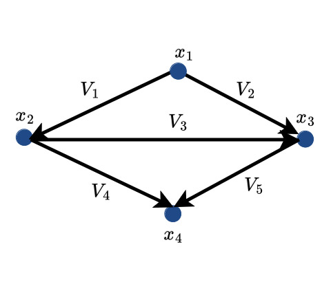
Now, instead of flows, let’s discuss about potential differences, or voltages, across nodes.

Solving $A^{\top} \vv x = \vv v$ tells us what potentials we need to put on the nodes to achieve the desired voltages. For example, the first row of $A^{\top} \vv x = \vv v$ is $-x_1 + x_2 = v_1$. This is Kirchoff’s Voltage Law!

Let’s start with Null$(A^{\top})$, which we find by setting $\vv v = \vv 0$.

From (8), Null$(A^{\top})$ is a line in $\mathbb{R}^4$ spanned by $\vv 1 = \bm 1 \\ 1 \\ 1 \\ 1\em$. The rank of $A$ must be $4 - 1 = 3$, which we saw was true above! This implies that we can increase the voltage across all nodes by the same amount, and achieve the same voltage drop between nodes. Makes sense!

The row space of $A$ is the column space of $A^{\top}$. There must be 3 independent columns of $A^{\top}$ (since rank = 3). So, let’s try to find them by inspection. The first three columns of $A^{\top}$ are

which can be verified to to be linearly independent. Therefore, only voltage configurations $\vv v$ lying in span$\{\vv v_1, \vv v_2, \vv v_3\}$ can be encoded on this graph. Therefore, for any $x_1$, $x_2$, and $x_3$, voltage configurations $x_1 \vv v_1 + x_2 \vv v_2 + x_3 \vv v_3$ are valid. Such configurations can be represented in code as follows.

We will understand where the statement in Exercise 1 comes from in the next couple of lectures!

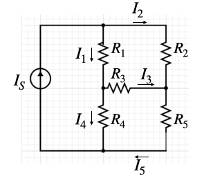
Using the current and voltage laws above, let’s try to compute the currents in a circuit consisting of a current source and several resistors. In particular, we will consider the below circuit:

We can verify that the above circuit conforms to the network flow depicted in Figure 1 by letting $I_S = s$, and $I_1, I_2, I_3, I_4, I_5 = f_1, f_2, f_3, f_4, f_5$. By the current law, we know that the currents must satisfy

for some numbers $c_1$ and $c_2$. Ohm’s law allows us to relate the current between two nodes and the voltage drop between two nodes as $V_i = I_i R_i$, where $R_i$ is the resistance of edge $i$. We may therefore write

where $R = \mathsf{diag}(R_1, R_2, R_3, R_4, R_5)$.

By the voltage law, $V_1, V_2, V_3, V_4, V_5$ is a consistent profile only if there exists some $x_1, x_2, x_3$ such that

Moving the terms involving $c_1$ and $c_2$ to the left side, we find that we must have

The left hand side may be expressed as a matrix, leading to the equation

We may verify that for positive $R_1, R_2, R_3, R_4, R_5$, the vectors $\vv v_1$, $\vv v_2$, $\vv v_3$, $R \vv f_1$, $R \vv f_2$ are linearly independent. Therefore, we may invert the matrix $\bm \vv v_1 & \vv v_2 & \vv v_3 & -R \vv f_1 & -R \vv f_2 \em$ to solve the above equation, from which we find that

Let’s try out some different resistances and check that the resulting current profiles make sense.

Does the above solution make sense? When all resistances are equal, the two branches of the circuit are equally appealing, so the current is split evenly. Let’s try a different resistance profile.

Now that the resistance $R_1$ is higher, the second path is prefereable. Therefore, a higher portion of the current flows through the second path. After bypassing the high resistance, some of the current reverts to the first path by flowing from node three to node two.